
Abstract
An extensive body of literature demonstrates how higher density leads to more efficient energy use and lower greenhouse gas (GHG) emissions from transport and housing. However, our current understanding seems to be limited on the relationships between the urban form and the GHG emissions, namely how the urban form affects the lifestyles and thus the GHGs on a much wider scale than traditionally assumed. The urban form affects housing types, commuting distances, availability of different goods and services, social contacts and emulation, and the alternatives for pastimes, meaning that lifestyles are actually situated instead of personal projects. As almost all consumption, be it services or products, involves GHG emissions, looking at the emissions from transport and housing may not be sufficient to define whether one form would be more desirable than another. In the paper we analyze the urban form–lifestyle relationships in Finland together with the resulting GHG implications, employing both monetary expenditure and time use data to portray lifestyles in different basic urban forms: metropolitan, urban, semi-urban and rural. The GHG implications are assessed with a life cycle assessment (LCA) method that takes into account the GHG emissions embedded in different goods and services. The paper depicts that, while the direct emissions from transportation and housing energy slightly decrease with higher density, the reductions can be easily overridden by sources of indirect emissions. We also highlight that the indirect emissions actually seem to have strong structural determinants, often undermined in studies concerning sustainable urban forms. Further, we introduce a concept of 'parallel consumption' to explain how the lifestyles especially in more urbanized areas lead to multiplication of consumption outside of the limits of time budget and the living environment. This is also part I of a two-stage study. In part II we will depict how various other contextual and socioeconomic variables are actually also very important to take into account, and how diverse GHG mitigation strategies would be needed for different types of area in different locations towards a low-carbon future.
Export citation and abstract BibTeX RIS

Content from this work may be used under the terms of the Creative Commons Attribution 3.0 licence. Any further distribution of this work must maintain attribution to the author(s) and the title of the work, journal citation and DOI.
1. Introduction
Radical greenhouse gas (GHG) reductions in the near future are needed to mitigate the climate change to a level adaptable for both human settlements and the environment (IPCC 2007). Since the majority of all the global GHG emissions seem to be related to urban settlements (Satterthwaite 2008, Dodman 2009, Hoornweg et al 2011), spatial planning has been argued to have significant potential to shape more sustainable human settlements (Carter and Fowler 2008, Fields 2009, Antrobus 2011). There is an extensive body of literature demonstrating how higher density offers opportunities for more efficient energy use and lower GHG emissions from transport and housing (Norman et al 2006, VandeWeghe and Kennedy 2007, Jenks and Burgess 2000, Ewing and Cervero 2010, Glaeser and Kahn 2010, Fuller and Crawford 2011).
On the other hand, increased volume of economic activity is claimed as another effect of urbanization. Agglomeration economies have for a long time explained how denser agglomerations are able to create more wealth (Ciccone and Hall 1996, Broersma and Oosterhaven 2009). This generally leads to more consumption with associated environmental burdens. In addition, different forms of agglomeration open up certain possibilities of consumption and undermine others, which is likely to affect the lifestyles. In fact, some recent evidence would indicate that, even where higher urban density leads lower private vehicle usage and housing energy needs, the life in denser agglomerations may be more consumption intense up to the point where the overall emissions exceed those caused by residents of less dense areas (Sovacool and Brown 2010, Heinonen 2012, Lenzen et al 2004).
There thus seems to be a gap in our current understanding on the urban form–GHG emission relationship, namely how the urban form affects lifestyles and thus GHGs on a much wider scale than traditionally assumed. Looked at from the perspective of research focusing on energy requirements and environmental burdens related to different lifestyles, the tradition is long (e.g. Schipper et al 1989, Biesiot and Moll 1995, Biesiot and Noorman 1999, Wier et al 2001, Bin and Dowlatabadi 2005, Brännlund and Ghalwash 2008, Cayla et al 2011), but the variables concerned rarely include the urban form. Some of this literature, especially the carbon footprint assessments based on monetary expenditure data (e.g. Baiocchi et al 2010; Kerkhof et al 2009; Hertwich and Peters 2009; Hertwich 2011; Erickson et al 2012; Heinonen and Junnila 2011a) bring consumption closer to the spatial location, yet mostly without trying to explain how the form affects the consumption choices. Still, studies in this field have demonstrated, e.g., that a life cycle perspective and consumption based approach are actually mandatory to fully understand the emissions related to a certain society because of the outsourced emissions, that is, the emissions embodied in all the consumed goods that are produced elsewhere and imported (Peters and Hertwich 2008, Ramaswami et al 2008, Schulz 2010).
Monetary expenditure data alone may also give an insufficient picture of the actual lifestyles (Schipper et al 1989). Most consumption, be it services or products, involves phases of use in everyday life reflected in time allocation of a consumer. Hence, it has been claimed that time use data contribute to better understanding of consumption patterns and changes therein (Gershuny 1987, Minx and Baiocchi 2009). Further, together monetary expenditure and time use data can give us understanding of the actual lifestyles of certain consumers and thus a possibility to understand the urban form–lifestyle relationships.
Drawn from the above discussion, the purpose of this paper is to analyze the urban form–lifestyle relationships and the resulting GHG implications. We employ both monetary expenditure and time use data to portray lifestyles in different basic urban forms in Finland: metropolitan, urban, semi-urban and rural. The GHG implications are assessed with a life cycle assessment (LCA) method that takes into account the GHG emissions embedded in different goods and services. We analyze first the consumption patterns of the residents in selected urban forms and calculate the associated GHGs, and then proceed to time use data to understand in more detail how and where the money is consumed.
There are some studies that have addressed the issue of how the urban form might affect the environmental burdens (Høyer and Holden 2003, Holden 2004, Holden and Norland 2005), but the tradition is relatively thin. To our knowledge this letter (1) brings valuable actual data based evidence to the discussion, and (2) is the first concentrating on a climate change perspective.
We present in the letter that, while the direct structural factors, transportation and housing energy, seem to follow the patterns reported in numerous studies and decrease with higher density, the reductions may actually be rather small and can thus be easily overridden by sources of indirect GHG emissions. We also highlight that the indirect emissions actually seem to have strong structural determinants, often undermined in studies concerning sustainable urban forms. We introduce a concept of parallel consumption to explain how certain lifestyles lead to multiplication of consumption outside of the limits of time budget and the living environment, e.g. using a multitude of service spaces while possessing a home with similar possibilities. We also look for contextual factors, such as time spent in traffic, for describing actual fuel consumption better than the average mileage driven. The findings indicate that much deeper understanding on the urban form–lifestyle relationships is needed in order to create truly effective urban planning strategies from the climate change perspective.
The structure of the letter is as follows. In section 2 the concept of situated lifestyles is defined. Section 3 explains the data and the utilized methods. In section 4 we analyze concurrently the lifestyles based on monetary consumption patterns, time use and the resulting GHGs. Section 5 looks at the lifestyles through the concept of parallel consumption. Finally, in section 6 the results are discussed and some final conclusions are drawn.
2. Situated lifestyles
Frequently, lifestyles have been seen as a product of the values of individuals (e.g. Bauman 2000, Firat and Dholakia 1998, Bin and Dowlatabadi 2005). Hence there is little need to consider the urban form as a determinant of individual behavior. There are other interpretations of lifestyles that take structures into account and argue that consumption is constrained by the surrounding structure. Baiocchi et al (2010) put emphasis on the physical location and residence of consumers. Yet, the variables they use are still to a large extent based on class, occupation and education. Schipper et al (1989) and Jalas (2002) go further to argue for paying attention to the activities and the locations of consumption. Spaargaren and Van Vliet (2000) has proposed a combination of the above, arguing that sociotechnical structures do most of the choosing for us, but that nevertheless consumers look for consistent 'style' across areas of consumption.
This study is premised on the claim that the form of a human settlement is a fundamental structural factor that underlies patterns of consumption. It affects housing types, commuting distances, availability of different goods and services, social contacts and emulation, and the alternatives for pastimes. Urban form thus is reflected in behavioral patterns, time allocation and purchasing decisions. We use the notion of situated lifestyles to capture this effect. We recognize other determinants of behavior, but argue that urban form affects time allocation as well as purchasing decisions deeply enough to create identifiable lifestyles even on a very highly aggregated level, and thus give an indication on how the urban form affects the GHG emissions.
3. Data and utilized methods
3.1. Four types of urban form
We utilize a setting of four different types of urban form in Finland to analyze the time use and consumption behavior and their GHG implications. The selection is based on the 'Statistical grouping of municipalities' of Statistics Finland3 that divides the country into three categories of urban forms according to the proportion of the residents living in urban areas and the size of the largest urban settlement: rural municipalities, semi-urban municipalities and cities. In addition, Helsinki metropolitan area (HMA) is separated from cities to form its own entity. Table 1 presents the analyzed groups and their characteristics.
Table 1. The main characteristics of the four types of area.
| Group/characteristics | HMA | Urban municipalities | Semi-urban municipalities | Rural municipalities |
|---|---|---|---|---|
| Definition (stat.fi) | Four cities: the capital Helsinki and its neighbors Vantaa, Espoo and Kauniainen. The area's total population is about one million and it forms an inseparable entity of workplaces, public transport etc | 'Municipalities in which at least 90% of the population lives in urban settlements or in which the population of the largest urban settlement is at least 15 000' | 'Municipalities in which at least 60% but less than 90% of the population lives in urban settlements and in which the population of the largest urban settlement is at least 4000 but less than 15 000' | 'Municipalities in which less than 60% of the population lives in urban settlements and in which the population of the largest urban settlement is less than 15 000; and those in which at least 60% but less than 90% of the population lives in urban settlements and in which the population of the largest settlement is less than 4000' |
| Family size | 1.93 | 2.05 | 2.27 | 2.33 |
| Annual per capita disposable income (€) | 22 000 | 16 200 | 15 700 | 14 100 |
| Housing types | ||||
| Apartment (%) | 72 | 60 | 32 | 14 |
| Terraced/detached (%) | 28 | 40 | 68 | 86 |
| Heating modes | ||||
| Electricity (%) | 13 | 21 | 28 | 36 |
| District heat (%) | 81 | 60 | 29 | 14 |
| Wood (%) | 0 | 3 | 11 | 18 |
| Other (%) | 6 | 16 | 32 | 32 |
| Living space per capita (sqm) | 39 | 40 | 46 | 44 |
| Population density (residents per km2)* | 1327 | 83 | 16 | 5 |
3.2. Consumption and time use data
We employ two primary data sources to analyze the lifestyles of the average residents of each type of area: the Household Budget Survey and the Time Use Survey of Statistics Finland. We utilize the most recent Household Budget Survey from 2006. The one-period cross-section data consists of 4007 households. The very detailed consumption expenditure data are classified according to the COICOP system4. Data comprise information from diary and interview parts of the survey. The diary part should give fairly reliable estimates for the ordinarily consumed goods and services, whereas the interview part increases the reliability of the data concerning the less frequent expenses, such as a purchase of a car, that are reported from the preceding 12 months in the interview. The data also contains background and income information for each household. Being a sample study, the data contains weight coefficients equal to the inverse probability of being sampled, and we take advantage of these probability weights when analyzing the data. The data describe private consumption only in monetary terms, and does not have information about prices or amounts purchased. Also, use of public goods, in Finland including schooling and health care for the most part, is not taken into account.
We made one enhancement to the data. We disaggregated the housing charges of apartment buildings into heating, electricity, maintenance and other according to statistics on housing management fees published by Statistics Finland (2009). According to the data, in HMA 30% and in the rest of Finland slightly over 40% of housing charges are actually communal energy payments and over 50% maintenance and repair payments. Thus, if not separated, analyses may lead to a false impression of very low energy usage for apartment building residents. In rented dwellings the rental payments were first disaggregated to housing charges and the rest according to average housing charges in each area, and then the housing charge share further according to the above description.
Time use surveys are, likewise, based on representative samples. The data used in this study were collected in the years 2009 and 2010. They involve 4410 individuals, aged above 10, reporting the course of altogether 7480 individual days. These diaries record the activity of the respondent in 10 min intervals for a 24 h period according to a classification scheme of 146 different activities accompanied by location data as well. In addition to the diaries, there are a large number of background variables that include indices of urban form.
3.3. GHG implication assessment
The GHGs are assessed for an average resident of each of the four types of area with an environmentally extended input–output life cycle assessment (EE IO LCA) model. IO methods provide comprehensiveness that would be impossible to reach with the process LCA approach regarding complex systems such as overall consumption. The IO method includes the whole economy, and using sectorial monetary transaction matrices describes the transactions between all the sectors to produce a certain outcome in one sector without truncation errors from system boundary selection (e.g. Suh et al 2004, Tukker and Jansen 2006). The method is very effective in accounting for emissions based on consumption activity as in this study. With the IO LCA approach the emissions from consumption of goods and services can be effectively allocated to the consumer regardless of the location of the consumption. The method is also relatively quick and assessments are simple to conduct and repeat while still in accordance with the ISO guidelines (Suh et al 2004).
As the IO application we employ a model called ENVIMAT developed for the Finnish economy (Seppälä et al 2011). We utilize the 2005 consumer-price version of the model, that has 52 sectors, classified according to the COICOP classification. Each sector thus returns the lifecycle GHG emissions per € used to the sector. The impacts are assessed as CO2 equivalents for GHG emissions according to IPCC's instructions (IPCC 1997). To create the consumer carbon footprints, we combine the emission intensities derived from ENVIMAT with Household Budget Survey data.
The data-model fit is perfect in theory as both utilize the COICOP classification system. The Household Budget Survey data were thus aggregated to the level of the 52 sectors of the assessment model. The sectors and their per euro GHG intensities are presented in table 2 in section 4 along with the monetary input to each sector and the assessment results. Some minor modifications to the model were still necessary in the aggregation process, however. First, in cooperation with the developers of the model5 we modified the intensity of sector CO455, district heat and hot water charges, etc, due to an identified calculation error in the model. Second, we separated own and purchased firewood and utilized the corresponding ENVIMAT sector only for the purchased share. The emissions from processing own wood to logs are reflected elsewhere in the consumption data as machinery and fuel expenses, and the combustion of wood can be argued to have zero net GHG impact. Finally, we employed a price level correction factor of 0.82 according to the data of Statistics Finland for the GHGs from actual and imputed rentals in HMA to avoid bias from higher housing prices.
Table 2. Consumption in the 12 COICOP main categories and in the 52 ENVIMAT sectors together with the resulting GHG emissions. (Note: 'n.e.c' stands for 'not elsewhere classified'.)
| COICOP | Monetary consumption (€ a−1) | Intensity | Overall GWP (kg a−1) | |||||||
|---|---|---|---|---|---|---|---|---|---|---|
| C01–12—individual consumption expenditure of households | HMA | Cities | Semi-urban | Rural | kg GHG/€ | HMA | Cities | Semi-urban | Rural | |
| C01—food and non-alcoholic beverages | 1961 | 1772 | 1818 | 1731 | 1692 | 1536 | 1575 | 1506 | ||
| C011 | Food | 1806 | 1628 | 1677 | 1606 | 1583 | 1436 | 1476 | 1418 | |
| C011a | Food: vegetal food products | 1007 | 888 | 920 | 870 | 0.7 | 705 | 622 | 644 | 609 |
| C011b | Food: products with animal contents | 798 | 740 | 756 | 736 | 1.1 | 878 | 814 | 832 | 809 |
| C012 | Non-alcoholic beverages | 156 | 144 | 141 | 125 | 0.7 | 109 | 100 | 99 | 88 |
| C02—alcoholic beverages and tobacco | 440 | 327 | 347 | 293 | 132 | 98 | 104 | 88 | ||
| C021+C022 | Alcoholic beverages + tobacco | 440 | 327 | 347 | 293 | 0.3 | 132 | 98 | 104 | 88 |
| C03—clothing and footwear | 809 | 563 | 459 | 355 | 324 | 225 | 183 | 142 | ||
| C031+32 | Clothing + footwear | 809 | 563 | 459 | 355 | 0.4 | 324 | 225 | 183 | 142 |
| C04—housing, water, electricity, gas and other fuels | 4446 | 3439 | 3285 | 2702 | 4043 | 3789 | 3684 | 3298 | ||
| C041 | Actual rentals for housing | 836 | 525 | 284 | 200 | 0.4 | 273 | 210 | 114 | 80 |
| C042 | Imputed rentals for housing | 2192 | 1694 | 1908 | 1498 | 0.4 | 717 | 678 | 763 | 599 |
| C043+44 | Maintenance and repair of the dwelling + water supply and miscellaneous services relating to the dwelling | 781 | 576 | 408 | 308 | 0.7 | 546 | 403 | 286 | 216 |
| C0451 | Electricity | 302 | 326 | 378 | 407 | 3.2 | 966 | 1043 | 1210 | 1302 |
| C0453 | Liquid fuels | 41 | 65 | 102 | 91 | 6.9 | 283 | 447 | 703 | 629 |
| C0454101 | Paid firewood and other fuels | 1 | 7 | 20 | 19 | 2.5 | 3 | 17 | 50 | 48 |
| C0454102+103 | Firewood, etc: own or benefit in kind | 8 | 21 | 58 | 82 | 0 | — | — | — | — |
| C0455 | District heat and hot water charges, etc | 285 | 225 | 127 | 96 | 4.4 | 1254 | 990 | 559 | 422 |
| C05—furnishings, household equipment and routine household maintenance | 886 | 707 | 724 | 619 | 377 | 301 | 311 | 266 | ||
| C051+C053 | Furniture and furnishings, carpets and other floor coverings + household appliances | 521 | 388 | 390 | 318 | 0.4 | 208 | 155 | 156 | 127 |
| C052+C054 +C055 | Household textiles + glassware, tableware and household utensils + tools and equipment for house and garden | 229 | 187 | 213 | 186 | 0.5 | 114 | 93 | 106 | 93 |
| C056 | Goods and services for routine household maintenance | 137 | 132 | 122 | 114 | 0.4 | 55 | 53 | 49 | 46 |
| C06—health | 579 | 500 | 500 | 424 | 172 | 158 | 150 | 135 | ||
| C061 | Medical products, appliances and equipment | 280 | 288 | 249 | 254 | 0.4 | 112 | 115 | 100 | 101 |
| C062+C063 | Outpatient services + hospital services | 300 | 212 | 251 | 170 | 0.2 | 60 | 42 | 50 | 34 |
| C07—transport | 2318 | 2133 | 2285 | 2310 | 1679 | 1683 | 1847 | 2030 | ||
| C0711 | Motor cars | 1169 | 1050 | 1136 | 1037 | 0.2 | 234 | 210 | 227 | 207 |
| C0712 | Motorcycles, snow mobiles, etc | 17 | 49 | 79 | 163 | 1.4 | 23 | 69 | 110 | 228 |
| C0713 | Bicycles | 21 | 19 | 26 | 14 | 0.3 | 6 | 6 | 8 | 4 |
| C072 | Operation of personal transport equipment | 653 | 806 | 939 | 1000 | 1.5 | 979 | 1209 | 1408 | 1499 |
| C0731 | Passenger transport by railway in Finland | 54 | 48 | 27 | 13 | 0.6 | 32 | 29 | 16 | 8 |
| C0732 | Passenger transport by road in Finland | 243 | 92 | 43 | 45 | 0.8 | 194 | 73 | 34 | 36 |
| C0733 | Passenger transport by air | 141 | 54 | 26 | 29 | 1.3 | 184 | 70 | 34 | 38 |
| C0734 | Passenger transport by sea and inland waterway | 18 | 10 | 6 | 6 | 1.4 | 25 | 15 | 8 | 8 |
| C0735 | Other purchased transport services | 3 | 5 | 4 | 2 | 0.4 | 1 | 2 | 2 | 1 |
| C08—communication | 470 | 403 | 380 | 373 | 94 | 81 | 76 | 75 | ||
| C08 | Communication | 470 | 403 | 380 | 373 | 0.2 | 94 | 81 | 76 | 75 |
| C09—recreation and culture | 2192 | 1558 | 1460 | 1274 | 1051 | 710 | 676 | 589 | ||
| C091 | Audio-visual, photographic and information processing equipment | 359 | 323 | 244 | 194 | 0.4 | 144 | 129 | 98 | 77 |
| C092 | Other major durables for recreation and culture | 217 | 75 | 97 | 114 | 0.8 | 173 | 60 | 78 | 91 |
| C093 | Other recreational items and equipment, gardens and pets | 312 | 281 | 302 | 261 | 0.6 | 187 | 169 | 181 | 157 |
| C094 | Recreational and cultural services | 589 | 412 | 390 | 350 | 0.2 | 118 | 82 | 78 | 70 |
| C095 | Newspapers, books and stationery | 357 | 259 | 251 | 227 | 0.4 | 143 | 104 | 100 | 91 |
| C096 | Package holidays | 358 | 208 | 177 | 128 | 0.8 | 287 | 166 | 142 | 103 |
| C10—education | 60 | 24 | 21 | 24 | 18 | 7 | 6 | 7 | ||
| C10 | Education | 60 | 24 | 21 | 24 | 0.3 | 18 | 7 | 6 | 7 |
| C11—restaurants and hotels | 910 | 617 | 503 | 364 | 377 | 254 | 208 | 151 | ||
| C111 | Catering services | 777 | 549 | 432 | 314 | 0.4 | 311 | 220 | 173 | 125 |
| C112 | Accommodation services | 132 | 68 | 71 | 50 | 0.5 | 66 | 34 | 36 | 25 |
| C12—miscellaneous goods and services | 2522 | 2093 | 2000 | 1711 | 947 | 730 | 665 | 565 | ||
| C121 | Personal care | 378 | 300 | 247 | 193 | 0.4 | 151 | 120 | 99 | 77 |
| C123 | Personal effects n.e.c. | 160 | 134 | 163 | 130 | 0.4 | 64 | 53 | 65 | 52 |
| C124 | Social welfare services | 134 | 109 | 100 | 72 | 0.2 | 27 | 22 | 20 | 14 |
| C125 | Insurance | 323 | 346 | 405 | 374 | 0.2 | 65 | 69 | 81 | 75 |
| C126 | Bank and financial services | 476 | 391 | 352 | 265 | 0.3 | 143 | 117 | 106 | 79 |
| C127 | Other services n.e.c. + items outside consumption expenditure | 595 | 552 | 548 | 518 | 0.3 | 179 | 166 | 164 | 155 |
| P312Y | Consumption n.e.c. abroad | 456 | 260 | 186 | 160 | 0.7 | 319 | 182 | 130 | 112 |
| Total | 17 593 | 14 135 | 13 782 | 12 177 | 10 906 | 9571 | 9486 | 8851 | ||
4. Purchasing patterns, time use and GHGs of the average consumers in the different types of area
Figures 1(A)–(C) present the overall results of the study in monetary purchases, GHGs and time use. Figure 1(A) show how the structure of consumption is surprisingly similar in all the samples, but the overall consumption levels increase from 12 200€ a−1 in rural areas to 13 800€ a−1 in semi-urban areas, 14 100€ a−1 in cities and 17 600€ a−1 in HMA. This indicates that the consumption patterns are actually quite different. All the consumers make the choices under the same time constraint, and thus time allocation needs to change to allow the overall higher consumption. Figure 1(C), depicting the daily allocation of time in the four types of area, shows that time use is in fact different. The important lifestyle related difference in time use patterns is the amount of leisure time spent outside of home. Leisure time spent outside of home varies from 8.7 h in HMA to 8.4 h in cities, 7.6 h in semi-urban areas and 6.6 h in rural areas. Thus, while the housing prices increase along with the level of urbanization (see section 3 also) and more money is spent on housing in the more urbanized areas, less time is spent at home and more actually allocated to taking advantage of the better service levels of the area. Figure 1(C) also shows that the higher income level in the more urbanized areas is mainly a result of higher salaries, as working time is very evenly distributed across the different urban forms.
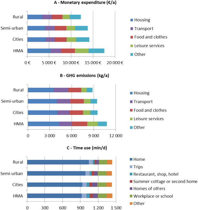
Figure 1. (A) The structure of monetary consumption, (B) GHGs and (C) time use distribution in the four types of area.
Download figure:
Standard imageThe increasing levels of monetary consumption and the data on how the time is allocated explain the GHG results of figure 1(B) that show increasing overall emissions towards the more urbanized areas, especially HMA. The overall carbon footprints, according to the assessment model, are 10 900 kg GHG a−1 in HMA, 9600 kg a−1 in cities, 9500 kg a−1 in semi-urban areas, and 8900 kg a−1 in rural areas. Thus, even though more services are consumed in the more urbanized areas, this does not solve the problem of increasing GHG emissions. The city type of living is actually not able to reduce even the emissions from housing and transport, as analyzed further in section 4.1, and thus the increased consumption of services only adds to the very similar large basis of emissions from the necessary consumption.
4.1. Transport related consumption patterns and GHGs
When analyzing the figures on a more detailed level, further evidence of how the type of area shows in the consumption patterns can be found. All the data are also comprised in tables 2–4 below. Starting from transport, our data show that higher density leads to lower fuel purchases related to private driving (category C072 in table 2) and resulting GHGs, which is in accordance with several earlier studies. However, the difference even between the two extremes, HMA and rural areas, is only 500 kg GHG a−1. One explanation, which has received little attention, is that the fuel efficiency is significantly weaker in cities. This reduces the differences in GHGs compared to kilometers driven. According to the Technical Research Centre of Finland the per kilometer emissions drop by almost a factor of two when moving to highways from city traffic (VTT 2012). This is also reflected in the time use data. More time is spent driving private vehicles in the less urbanized areas, but the difference between the highest and the lowest end is only around 20% (table 4).
Table 3. Time consumption based on daily activities.
| Activity | Time consumption (min d−1) | |||
|---|---|---|---|---|
| HMA | Cities | Semi-urban | Rural | |
| Gainful employment, total | 137.9 | 132.5 | 136.9 | 139.2 |
| Domestic work, total | 261.2 | 257.7 | 277.6 | 304.1 |
| Food preparation and kitchen work | 40.0 | 42.4 | 41.7 | 47.2 |
| Washing and ironing | 10.7 | 11.5 | 12.1 | 11.6 |
| Cleaning, heating, organizing and planning | 36.7 | 39.1 | 45.1 | 53.5 |
| House building, maintenance and repairing | 7.3 | 9.2 | 11.6 | 18.7 |
| Gardening and pets | 5.8 | 7.3 | 10.6 | 18.3 |
| Helping adult family member | 1.0 | 0.9 | 0.5 | 2.2 |
| Childcare | 21.8 | 15.0 | 19.2 | 13.4 |
| Shopping and services, total | 27.1 | 27.1 | 26.4 | 24.1 |
| Personal care, total | 649.7 | 651.3 | 654.6 | 650.8 |
| Sleeping | 518.5 | 519.3 | 522.9 | 521.3 |
| Meals | 81.3 | 83.9 | 78.6 | 84.9 |
| Washing and dressing | 50.0 | 48.1 | 53.1 | 44.6 |
| Study, total | 29.1 | 33.4 | 38.5 | 34.2 |
| Free time, total | 377.2 | 384.4 | 361.2 | 345.6 |
| Socializing with family and friends | 52.9 | 51.0 | 45.6 | 43.9 |
| Entertainment and culture | 6.7 | 6.4 | 4.2 | 4.5 |
| Resting | 13.9 | 16.5 | 19.6 | 20.6 |
| Participatory activity | 17.4 | 18.0 | 16.2 | 17.6 |
| Sports | 32.7 | 32.6 | 30.1 | 27.7 |
| Outdoor activities | 8.6 | 9.6 | 10.6 | 12.6 |
| Hobbies | 7.3 | 6.9 | 4.8 | 6.9 |
| Computer hobbies | 32.2 | 30.9 | 27.9 | 24.8 |
| Games and playing | 23.0 | 20.5 | 17.7 | 15.7 |
| Reading, radio and television | 182.5 | 191.8 | 184.5 | 171.2 |
| Travel, total | 79.9 | 66.0 | 66.7 | 61.7 |
| Travel to and from work | 16.1 | 11.8 | 11.3 | 10.6 |
| Other daily travel | 52.5 | 42.7 | 43.5 | 40.2 |
| Long distance travel | 11.3 | 11.5 | 11.9 | 10.9 |
| Unspecified | 15.9 | 20.2 | 15.0 | 19.4 |
| Total | 1440 | 1440 | 1440 | 1440 |
Table 4. Time use by locations.
| Location | Time use (min d−1) | |||
|---|---|---|---|---|
| HMA | Cities | Semi-urban | Rural | |
| Home | 922.3 | 935.2 | 985.5 | 1041.2 |
| Second home | 44.4 | 44.3 | 37.0 | 21.8 |
| Workplace or school | 148.2 | 145.8 | 149.8 | 130.6 |
| Visiting other home | 89.0 | 90.6 | 66.0 | 54.1 |
| Restaurant | 15.7 | 12.8 | 6.5 | 4.8 |
| Shop, mall, market | 22.7 | 20.2 | 20.3 | 17.8 |
| Hotel, camping site | 15.1 | 10.7 | 7.0 | 5.3 |
| Other (not a trip) | 97.4 | 103.6 | 92.2 | 95.1 |
| Trips total | 83.7 | 70.9 | 69.7 | 66.4 |
| Walking | 18.3 | 10.2 | 7.5 | 3.7 |
| Biking | 1.9 | 4.6 | 3.2 | 1.6 |
| Private motor vehicles | 36.1 | 42.0 | 45.7 | 48.2 |
| Taxi | 2.3 | 0.8 | 0.5 | 1.2 |
| Public transport | 16.0 | 6.2 | 5.0 | 4.5 |
| Air and maritime travel | 3.5 | 2.7 | 3.3 | 2.0 |
| Other | 5.7 | 4.3 | 4.5 | 5.4 |
| Total | 1439 | 1434 | 1434 | 1437 |
The overall resulting GHGs from transport vary even less between the areas, from roughly 2000 kg a−1 in rural areas to 1800 kg a−1 in semi-urban areas and 1700 kg a−1 in cities and in HMA. In monetary terms the difference is yet smaller, from approximately 2100€ a−1 in cities to 2300€ a−1 in all the other area types. What narrows the difference in both GHG and expenditures is that public transport, taxi use and air travel are more frequent in the more urbanized areas, especially in HMA. In our data air travel is actually largely embedded in the COICOP category 09, package holidays (C096 in table 2), which the HMA residents purchase much more as well. Overall, the finding that a decrease in car use is actually compensated by increased air travelling is similar to that reported by Ornetzeder et al (2008), especially when taking into account the emissions from package holidays.
The transport category in the assessment includes car purchases as well, or more precisely the emissions from car manufacturing. Our data comply with the finding of e.g. Ewing et al (2003) that fewer private cars are owned in denser areas, approximately 0.3 per capita in HMA compared to 0.4 in cities and 0.5 in semi-urban and rural areas. This does not give an advance in GHGs for the more urbanized areas, however, as higher affluence seems to lead to a higher share of the purchases targeting to new cars. Well over 50% of the overall expenditure on car acquisition is directed to new cars in HMA, but only 30%–40% in all the other area types.
4.2. Consumption on housing and the resulting GHGs
Figures 1(A)–(C) show how more time is spent at home in the less urbanized (1(C)) areas but how the residents in the more urbanized areas spend more money (1(A)) and cause higher GHG emissions (1(B)) related to housing activities (categories C04 and C05 in table 2), 4400 kg in HMA compared to 4100 kg in cities, 4000 kg in semi-urban areas and 3600 kg in rural areas. The primary explanation from our data is that the energy purchases are only slightly lower in cities, but the city residents spend much more on maintenance, appliances, furniture and home decoration. When the communal building energies in apartment buildings are divided between the residents and a per capita perspective is taken, the differences are only moderate, the energy purchases varying from approximately 580€ in HMA to 670€ in rural areas. An interesting notion from time use data is that, despite being at home much less, the HMA and city residents allocate the most time for entertainment technologies and computer games in both absolute and relative terms (table 3), meaning that the life at home in more urbanized areas can be more energy intensive despite the smaller apartments and less time spent at home.
The residents in the more urbanized areas also both possess more second homes and summer cottages, and spend more time occupying them, as depicted in figure 1(C) and in table 4. This further closes the gap in spending on energy, as the variation is only from 640€ in the denser areas to 700€ in more rural areas when all the possessed living spaces are taken into account (CO451–455 in table 2).
The differences in heating modes give arise to interesting notions. In HMA and in cities the dominant heating type is district heat, whereas in less urbanized areas significantly more expensive (in € kWh−1) electricity dominates heating (see table 1). The amount of wood used for heating also increases significantly towards the less urbanized areas. Thus, in HMA and in cities actually more kWh of housing energy are consumed. Measured in GHGs, the overall emissions are almost equal around 2500 kg a−1 in all the area types (CO451–455 in table 2).
The time use data depict again a couple of important differences in the lifestyles between the different types of area. The time allocated for repairs and maintenance varies from 7 min d−1 HMA to 19 min d−1 in rural areas. At the same time, the HMA and city residents spend much more money on maintenance and repairs. Thus, where these activities are executed by the residents themselves in the less urbanized areas, the residents in the more urbanized areas purchase them as services and thus actually buy more leisure time for themselves. The time use data also indicate that the home may serve slightly different needs. Especially in HMA, the residents spend much more on decoration, household textiles etc. While they spend much less time at home, as mentioned earlier, they visit the homes of others much more, approximately 90 min d−1 in HMA and in cities compared to 66 min d−1 in semi-urban areas and 54 min d−1 in rural areas. Thus the importance of showing tastefully decorated homes to visiting friends and relatives may be one explanation for the higher level of expenditure on housing goods.
4.3. Other consumption patterns and the GHG implications
The other consumption categories maybe reflect the daily lifestyle choices the most. While these have traditionally been left out of the analyses on the urban form related emissions, we depict here how affluence seems to show as the highest consumption in all the remaining consumption categories in HMA, pushing the emissions up as well as depicted in figure 1(B).
Figures 1(A) and (B) show how the purchases and the resulting GHGs from food, drinks and clothing increase towards the more urbanized areas. The purchases of food and drinks (C01, C02, table 2) have relatively little variation between the areas, mainly from slightly more wines, fruits and vegetables purchased in HMA. Most of the difference is thus explained by the purchases of clothes (C03), which vary from 810€ in HMA to 560€ in cities, 460€ in semi-urban areas and 360€ in rural areas. Table 4 depicts how the time spent in shops increases from 18 min d−1 in rural areas to 22 min d−1 in HMA, which gives some indication that higher purchases mean higher volume, not just differences in quality.
What reflects even more clearly how higher affluence and proximity to consumption opportunities shape the lifestyles is consumption of leisure goods and services. Almost twice as much money is spent by an average HMA resident on recreation and culture (C09 in table 2) as in rural areas. In particular, cultural services such as movies and theaters, swimming pools and courses and camps related to hobbies are purchased clearly the most in HMA, at 3100€ a−1 compared to 1600€ a−1 in rural areas. Cities and semi-urban areas position between the extremes, with slightly higher consumption in cities. The pattern continues to restaurants and hotels as well (C11 in table 2), where the differences are even higher. Also, significantly more time is spent utilizing these services in the more urbanized areas, as depicted in table 4, indicating differences in lifestyles. Overall, the GHG impacts from these consumption activities are quite significant, as the combined emissions from the categories C09 and C11 are almost 1500 kg for a HMA resident, nearly 15% of his/her annual carbon footprint, but in cities under 1000 kg, and only 880 kg in semi-urban areas and 740 kg in rural areas.
5. Emerging evidence on the phenomenon of parallel consumption
An aspect of urban agglomerations is the possibility of sharing resources and potentially reducing the existing size of personally owned assets, especially space. Smaller living spaces in more dense areas can be interpreted as a tradeoff between own and shared spaces. Laundries, parks, restaurants, cafés and pubs as extensions of the home are obvious examples. At best this could extend to sharing of equipment, household utilities etc and decrease the need to own goods. With this logic, many services can also contribute to eco-efficiency by reducing material and energy consumption (Halme et al 2004).
However, commercial services outside of home do not always lead to reduced overall material and energy use. It may well be that the usage and resource needs of all the 'shared spaces' exceed the gain from reduced own living space. Restaurants serve their clientele only for short hours per day and the sites of cultural events may be even less frequently uses by their clients, which increase their GHG intensity per used service. Dense urban living may also create needs for summer cottages and second homes, particularly when such an arrangement is affordable, which further increase one's actual space needs. Summer cottages are also often equipped with all modern machinery to reduce the need to carry things along when visiting the cottage and to make the place more pleasant. Equipment in the summer cottage may also increase the need for heating even when nobody is present. All this increases the GHGs that we cause even when we choose to live in smaller apartments in city centers.
We call this phenomenon here 'parallel consumption' and define it as concurrent consumption of service spaces in different locations. Our homes are heated and many electric appliances are run while we use diverse service spaces that extend our living space outside of the actual home. The concept aims to capture the way that consumption of space can multiply and extend beyond the apparent limit of time budgets or the spatial constraint imposed by the home or even the surrounding settlement. The concept also helps to depict that our actual home can only give a limited picture of the space that we actually use for living and thus what counts for the GHG impacts that we cause.
The phenomenon of parallel consumption is strongly present with service use such as hotels, cafés and restaurants, as homes are heated and operated at the same time, and also equipped to offer similar services. In HMA 31 min d−1 is spent in hotels and restaurants (table 4), in cities 24 min d−1, but only 14 min d−1 in semi-urban areas and 10 min d−1 in rural areas. Correspondingly, 910€ a−1 is spent for these services by the average resident of HMA (table 2), 620€ a−1 in cities, 500€ a−1 in semi-urban areas and 360€ a−1 in rural areas. Concerning second homes the pattern is similar.
In the case of summer cottages and second homes, the parallel consumption phenomenon is continuous as two living spaces are concurrently in possession of those owning such premises. The consumption statistics show that in Finland 25% of the households in HMA possess a summer cottage, 22% in cities, 23% in semi-urban areas and 20% in rural areas, which depicts that also in this respect smaller living spaces are actually compensated by spaces elsewhere. Also, persons living in HMA and in cities have the highest time use in summer cottages with 44 min d−1 compared to 37 min d−1 in semi-urban areas and 22 min d−1 in rural areas. As was depicted in section 4, this closes down the advantage in housing energy consumption of more dense living. Energy purchases for the summer cottages and second homes vary from approximately 60€ a−1 by the HMA residents to 40€ a−1 in cities and in semi-urban areas and 30€ a−1 in rural areas. Possession of summer cottages may also relate to owning of private vehicles, since the vast majority of all the trips to summer cottages are made with private cars (Perrels and Kangas 2007). This hinders the full materialization of the potential of lower private driving needs in more dense agglomerations.
Movie theaters, swimming halls, spas, gyms, laundries etc have similar qualities, extending our living space to different locations. According to both monetary expenditure and time use data sets, the higher affluence level and higher service level in more urbanized areas lead to increased utilization of these services, followed by increased GHGs. When recognizing that many of the services where parallel consumption materializes depend on dedicated single-purpose space, parallel consumption highlights the 'hidden' burden of services and the logic of how service space gets included in the carbon footprints of individual consumers.
6. Discussion and conclusions
According to the purpose of the paper, we have demonstrated how there seem to be identifiable and from a GHG perspective significant urban form related lifestyle differences between the residents of different types of area even on a very aggregate level, making lifestyles actually situated instead of being mere personal projects. In a case study of Finland we found that even though the emissions related directly to the urban form, those from housing energy and private driving fuel combustion, decrease along an increase in the level of urbanization, when all the indirect emissions related to these categories were taken into account, in housing more emissions seem to be caused in the more urbanized areas and in transport the differences are significantly reduced, as shown by table 2. Furthermore, the more urbanized area types seem to associate with more GHG intensive lifestyles concerning emissions from other consumption activities. As indications of the consumption intensive urban lifestyles we pointed out for example that clothes and electronics are bought much more in the more urbanized areas, and that especially in all kinds of leisure service the consumption increases significantly along with the degree of urbanization. In addition, while in the less urbanized areas the daily life is much more home centered based on their time allocation, the smaller homes are at least equally equipped in cities, while more time is allocated to consuming services outside the home.
The overall carbon footprint of an average resident in HMA in Finland is 10,900 kg a−1 according to the study, followed by city and semi-urban areas with 9600 kg a−1 and 9500 kg a−1 respectively and rural areas with 8900 kg a−1. Consistently with the income hypothesis of agglomeration economies (e.g. Ciccone and Hall 1996), the first explanation is the higher affluence level in the more urbanized areas that seems to result in higher consumption. However, it seems that the urban type of living cannot very effectively reduce even the emissions related to the home or transport. Although a higher share of the overall purchases in more urban areas is allocated to services with lower GHG intensities, there is a very similar large basis of necessary consumption (housing, transportation and food) and emissions in each area. Thus the higher consumption volume only adds to the emissions instead of redirecting the whole consumption towards low GHG intensity activities. On the other hand, the overall GHG intensity of consumption decreases towards the more urbanized areas due to the increase in consumption of services from the lower end of GHG intensities of different commodity groups.
Based on the evidence on how we tend to extend our living space from the actual home to all kinds of service space while still equipping our homes to produce similar services, we brought into discussion the concept of parallel consumption. This phenomenon is not bound to any single urban form, but it would seem that the more urban lifestyles are more strongly based on this type of consumption, where reduced living spaces are actually compensated by service space use outside of the actual home. Increased use of summer cottages may indicate also that the hectic city lifestyle encourages possessing such spaces for more peaceful moments. Overall, the time use data showed that as much as 120 min d−1 more of the time outside of workplace or school is spent at home in rural areas compared to the more urbanized areas of HMA and cities. As this difference is largely spent for consumption of services outside of the actual home, the concept of parallel consumption helps in explaining the finding that the more urban lifestyles seem to lead to the highest GHG loads. As a worst case scenario, the study also points out that living is still relatively home centered in Finland, and thus significant growth in the parallel consumption phenomenon is possible in the future. On the other hand, economic crises and the current trend of decreasing economic growth presumably constrain the scope for parallel consumption.
The study includes uncertainties that can be divided into three broad categories. First, both data sets are subject to errors and biases, especially regarding the less frequently occurring activities or purchased goods. We tried to avoid this type of problem by using primarily aggregated data, especially concerning less frequently purchased goods. Also, the 52 category aggregation of the ENVIMAT assessment model forced us to avoid the most detailed data. These problems relate to sample sizes as well, small samples increasing the uncertainty. In this study the samples remained rather large with over 500 observations in each sample. However, it is well known that people tend to underreport monetary amounts used in socially undesirable sectors such as alcohol (e.g. Kok et al 2006). In the employed Finnish data the situation is relatively good, as the consumption estimates from consumer expenditure survey cover 87% of the consumption data in the national accounts (70 285 and 80 439 m€). Further, according to the consumer survey user's handbook (Statistics Finland 2006), this is due to differences in the accounting principles and thus the difference cannot be considered very significant. Furthermore, as the data are formed by combining diary and interview data their precision is quite high; standard errors in all the main consumption categories with the exception of spending on education are less than four per cent (Statistics Finland 2006).
The second source of uncertainty is the IO LCA method itself and thus the ENVIMAT assessment model. While IO LCAs are argued to be the most suitable for wide system level assessments in the built environment (Crawford 2011), they do have some problems. The primary source of uncertainty arises from the aggregation error inherent to all IO models (e.g. Wiedmann 2009). In ENVIMAT there are only 52 sectors, meaning that relatively diverse production sectors and individual products are inevitably aggregated together and given one single emission factor. This leads to another problem in IO LCAs, namely proportionality and homogeneity assumptions. These mean the straightforward assumption of IO approach that the monetary purchases would be linearly proportional to the output (GHGs) (e.g. Treloar 1997). The significance of this problem can be diminished by concentrating on the average consumers, as in this study. With sufficient samples the average consumers should use average goods and the problem would not be significant. Notwithstanding, Girod and De Haan (2010) have provided evidence that the products purchased by the more affluent consumers are not average products and that the monetary differences actually reflect differences in quality instead of quantity. In this case it might be that the IO LCA overestimates the emissions of the more affluent consumers, which would decrease the differences between the areas in this study. However, this concerns mainly the daily consumption of goods and that of some durable goods, but a large part of the consumption activity targets to exactly the same goods and services. Overall, the GHG assessment related problems are also reduced, as the paper describes the lifestyle differences from two other data sets as well. Regarding the GHG results, Heinonen and Junnila (e.g. Heinonen 2012) have also tested earlier that the results of the ENVIMAT model are very similar to those of another IO model, EIO LCA (Carnegie Mellon University 2008), in the Finnish context.
Concerning the possible price and currency level asymmetries between the data and the model, the fit is excellent, since both ENVIMAT and the Household Budget Survey are based on the same CIOCOP classifications, and the 2006 Household Budget Survey that we utilize has been employed in building the ENVIMAT model. Further, in ENVIMAT the often problematic domestic technology assumption of the majority of IO LCAs is relaxed and the imports from the most important trade partners of Finland are taken into account (Seppälä et al 2011).
Another uncertainty perspective arises from the assumptions regarding energy. In this study we have assumed that the same average energy (from ENVIMAT) is used in all the areas. If the local energy production in a certain area were much more or less GHG intensive than the Finnish average, it would affect the carbon footprints significantly. From 23% (HMA) to 27% (rural areas) of the carbon footprint comes from just the housing energy, and the local energy profile affects the local services and locally produced goods as well. Now, in HMA the local energy production is actually very similar in GHGs to the Finnish average and the other three area types consist of locations from all around Finland. Thus the results of the study in general are not subject to this error, but within cities, semi-urban areas and rural areas there exist locations where the local energy production deviates significantly from the national average. Heinonen and Junnila demonstrate the impact comparing Helsinki to Porvoo (Heinonen and Junnila 2011b), which belongs to cities in the samples of this study, but actually has a very different energy production profile from the Finnish average.
Furthermore, district heat can be seen as a byproduct of electricity generation. The employed assessment model ENVIMAT follows the shared benefits method, meaning that primary energy use is allocated according to the need to produce a similar amount of heat or electricity separately. The sensitivity of the results to the method of dividing the emissions of combined heat and power (CHP) production is rather high, as the production in Finland is predominantly fossil-fuel based. Allocating more emissions to electricity would result in lower emissions for the city residents using primarily district heat for heating purposes.
Finally, the paper presents a case study of Finland, which sets limitations for the generalizability of the results. In other locations around the globe different factors may dominate the emissions, which could significantly change the outcome of a similar analysis. The phenomenon of parallel consumption is present in all types of urban setting, and the role of indirect emissions is certainly important in all the developed countries with high consumption volumes. However, the differences in housing energy use and private driving etc, dominant factors in the GHG emissions, may be much larger in other contexts and lead to different conclusions.
To conclude, as part I of a broader study, the purpose of the study was to describe the broad context and depict that the urban form impact is deep enough to show in carbon footprints even on a highly aggregated area type division. On a more detailed level there is actually a large variation of different kinds of urbanization within each of these area types and a diverse set of lifestyles. These present thresholds where a certain other impact is greater than that of the urban form, for example that of local energy production. Even in these, the urban form shapes the lifestyles, but understanding the connections in a more detailed level is imperative to materialize the potential of designing location specific GHG mitigation strategies. In part II we will focus on these variables that affect the GHGs when one step deeper from purely urban form is taken.
Footnotes
- 3
Statistics Finland: Statistical grouping of municipalities, available at http://stat.fi/meta/kas/til_kuntaryhmit_en.html (25 October 2012).
- 4
UN: Classification of Individual Consumption according to Purpose, available at http://unstats.un.org/unsd/cr/registry/regcst.asp?Cl=5 (25 October 2012).
- 5
Telephone conversation: Jukka Heinonen–Tuomas Mattila, 9 November 2012.