
Abstract
We have investigated the spatio-temporal carbon balance patterns resulting from forcing a dynamic global vegetation model with output from 18 climate models of the CMIP5 (Coupled Model Intercomparison Project Phase 5) ensemble. We found robust patterns in terms of an extra-tropical loss of carbon, except for a temperature induced shift in phenology, leading to an increased spring uptake of carbon. There are less robust patterns in the tropics, a result of disagreement in projections of precipitation and temperature. Although the simulations generally agree well in terms of the sign of the carbon balance change in the middle to high latitudes, there are large differences in the magnitude of the loss between simulations. Together with tropical uncertainties these discrepancies accumulate over time, resulting in large differences in total carbon uptake over the coming century (−0.97–2.27 Pg C yr−1 during 2006–2100). The terrestrial biosphere becomes a net source of carbon in ten of the 18 simulations adding to the atmospheric CO2 concentrations, while the remaining eight simulations indicate an increased sink of carbon.
Export citation and abstract BibTeX RIS

Content from this work may be used under the terms of the Creative Commons Attribution-NonCommercial-ShareAlike 3.0 licence. Any further distribution of this work must maintain attribution to the author(s) and the title of the work, journal citation and DOI.
1. Introduction
The terrestrial biosphere affects the atmospheric CO2 concentration ([CO2]) through uptake and release of CO2. On-going and projected future changes in climate and [CO2] have the potential, in turn, to impact the biosphere–atmosphere net carbon exchange and the relative size of its main component fluxes, net primary production (NPP)—normally an uptake of carbon from the atmosphere—and heterotrophic respiration (Rh), which returns carbon to the atmosphere, mainly through decomposition of organic residues. Carbon emissions from wildfires (Cfire) constitute an additional, globally much smaller, return flux (Denman et al 2007). The balance between these uptake and release fluxes (the net ecosystem exchange, NEE) determines whether the biosphere acts locally as a source or a sink for CO2 relative to the atmosphere. As climate and [CO2] changes, the magnitude and geographic distributions of sources and sinks will change, feeding back to the evolution of climate (Le Quéré et al 2009). Experimental (Norby et al 2005) and modelling studies (Cramer et al 2001, Hickler et al 2008) generally suggest that rising [CO2] will enhance NPP and ecosystem carbon storage, although the size and persistency of this effect is still debated (Hungate et al 2003, Thornton et al 2007, Hickler et al 2008). Rising temperatures have a more complex, geographically variable, impact, with a longer and warmer growing season tending to enhance productivity in boreal and temperate regions with ample moisture, while heat stress, soil water losses and increased respiration rates are more likely to reduce carbon storage in warm climate and water-limited ecosystems (Nemani et al 2003, Morales et al 2007, Ahlström et al 2012b). Modelling studies attempting to analyse the overall global impact of projected future climate change on terrestrial ecosystem carbon storage generally reveal large differences between models in terms of the size and even the sign of the net change in global NEE, as well as the geographic distribution of sources and sinks, (Cramer et al 2001, Friedlingstein et al 2006, Sitch et al 2008, Ahlström et al 2012a), although a majority of models suggest that the ability of the terrestrial biosphere to store carbon will ultimately decline with global warming under a 'business as usual' future emissions scenario (e.g. Cox et al 2000, Cramer et al 2001, Joos et al 2001, Friedlingstein et al 2006). Overall, uncertainties in terrestrial sources and sinks of CO2 in a future climate remain large, and contribute to the uncertainty in [CO2] and thereby climate itself.
The uncertainties in carbon uptake or release, and thereby the wide range of estimates that have been published, originate from a number of different sources. Dynamic global vegetation models (DGVMs; Cramer et al 2001, Sitch et al 2008) or Earth system models (ESMs; Friedlingstein et al 2006, Randerson et al 2009) differ in their projections of future terrestrial carbon storage due to different but plausible representations of the underlying processes. For example, the response of terrestrial carbon uptake to rising [CO2] is debated (e.g. Hungate et al 2003, Norby et al 2005, Hickler et al 2008) and its response to [CO2] has been shown to differ among a range of models (Cramer et al 2001).
Uncertainties in the forcing (changes in climate and/or atmospheric [CO2]) contribute to the uncertainties in terrestrial sources and sinks of carbon. Effects on C-balance of differences in climate forcing were compared by Scholze et al (2006), showing a large dependence on the temperature response of the climate model: larger temperature changes in the 21st century generally increased the tendency for the terrestrial biosphere to become a source of CO2 to the atmosphere. The variability in carbon storage caused by the choice of the climate model can be as large as or larger than the variability between e.g. different emissions scenarios (Morales et al 2005, Ahlström et al 2012a). Better understanding of the response of the terrestrial biosphere is important to narrow these uncertainties.
In this study, we employ an individual-based dynamic vegetation–ecosystem model to assess the uncertainty in terrestrial carbon uptake that is caused by uncertainty in the climate forcing. We applied climate output from simulations of the RCP 8.5 from 18 different coupled atmosphere–ocean general circulation models and earth system models (hereafter referred to as GCMs), all participating in the Coupled Model Intercomparison Project Phase 5 (CMIP5), as input to a vegetation model simulating the terrestrial carbon cycle, and analyse the spread in carbon uptake between the simulations, as well as the characteristics of regional responses. The large set of simulations enables determination of the key driving factors for the variability in carbon storage, and thereby for part of the uncertainty in future estimates of sources and sinks of carbon.
2. Methods
2.1. Ecosystem model description
Ecosystem carbon balance response to climate and [CO2] change were simulated with LPJ-GUESS, a dynamic vegetation–ecosystem model incorporating a detailed, individual- and patch-based representation of vegetation structure, demography and resource competition (Smith et al 2001). The detailed dynamics have been demonstrated to improve the realism of the model in simulating transient shifts and geographic patterns of vegetation and carbon balance (Smith et al 2001). LPJ-GUESS represents vegetation as a mixture of plant functional types (PFTs; supplementary material, tables S1 and S2 available at stacks.iop.org/ERL/7/044008/mmedia) that vary dynamically in response to the climate (temperature, precipitation, incoming shortwave radiation) and [CO2] forcing and the evolution (succession) of vegetation structure in each of a number (10 in our study) of replicate patches simulated for each 0.5° × 0.5° grid cell. Population dynamics (establishment and mortality) are influenced by current resource status, demography and the life-history characteristics of each PFT (Hickler et al 2004, Wramneby et al 2008). Individuals are represented for trees and are identical within an age-size cohort in each patch. Growth and competition for light and water among woody plant individuals and a grassy ground layer govern the initial structure, PFT composition and transient dynamics of vegetation in each patch. Photosynthesis, respiration, stomatal conductance and phenology are simulated on a daily time step. NPP accrued at the end of each simulated year is allocated to leaves, fine roots and stems according to a set of prescribed allometric relationships for each PFT (Sitch et al 2003), effecting height, diameter and biomass growth. Biomass-destroying disturbances are simulated as a stochastic process, here with a generic expectation of 0.01 yr−1. In addition, fires are modelled prognostically based on temperature, current fuel load and moisture (Thonicke et al 2001). Decomposition of plant litter and two soil organic matter pools follows first-order kinetics with dependency on soil temperature and moisture.
A detailed description of LPJ-GUESS is given by Smith et al (2001). Updates relative to the latter publication are described in Hickler et al (2012). The PFT set and parameters employed in this study are provided in the supplementary material, tables S1 and S2 (available at stacks.iop.org/ERL/7/044008/mmedia).
In this letter we analyse NEE, i.e. the net exchange of carbon between the terrestrial ecosystem and the atmosphere. NEE is here defined as the balance between gross primary productivity (GPP), the carbon assimilated through the process of photosynthesis, and the release fluxes of autotrophic (Ra) and heterotrophic (Rh) respiration as well as carbon released to the atmosphere through biomass burning by wildfires, Cfire. We also analyse changes in the total terrestrial (vegetation and soil) carbon pool (Cpool) which essentially corresponds to the accumulated NEE. In the present paper, all downward fluxes (atmosphere to biosphere) are denoted by a negative sign and all upward fluxes (biosphere to atmosphere) by a positive sign.
2.2. Input data and simulation protocol
We forced LPJ-GUESS with output from 18 AOGCMs and ESMs (table 1) participating in the Coupled Model Intercomparison Project Phase 5 (CMIP5) (Taylor et al 2011) under the RCP 8.5 representative concentration pathway (Riahi et al 2007). Our focus here is on assessing effects of variation in climate under a given [CO2] pathway on terrestrial carbon fluxes, which for LPJ-GUESS has been found to introduce larger variability than climate from a single GCM but using different [CO2] trajectories (Ahlström et al 2012a). All ESMs and GCMs used prescribed [CO2] forcing, hence the carbon cycle feedbacks, when available in a given model, were turned off. We acquired data from all GCMs for which complete series of historical and scenario data were provided in the CMIP5 repository as of April 2012. Because all climate data were bias corrected using CRU TS 3.0 1961–90 climatologies (Mitchell and Jones 2005), the monthly fields of precipitation, downward shortwave radiation and air temperature were bi-linearly interpolated to the CRU grid (0.5° × 0.5° resolution). For calculation of photosynthesis and water balance, temperature and shortwave radiation are interpolated to daily values and monthly precipitation is distributed using the number of rainy days per month (Smith et al 2001, Sitch et al 2003).
Table 1. CMIP5 models and modelling groups.
| Modelling centre (or group) | Institute ID | Model name |
|---|---|---|
| Canadian Centre for Climate Modelling and Analysis | CCCMA | CanESM2 |
| National Center for Atmospheric Research | NCAR | CCSM4 |
| Centre National de Recherches Meteorologiques/Centre Europeen de Recherche et Formation Avancees en Calcul Scientifique | CNRM-CERFACS | CNRM-CM5 |
| LASG, Institute of Atmospheric Physics, Chinese Academy of Sciences | LASG-IAP | FGOALS-s2 |
| NOAA Geophysical Fluid Dynamics Laboratory | NOAA GFDL | GFDL-CM3 GFDL-ESM2M |
| NASA Goddard Institute for Space Studies | NASA GISS | GISS-E2-R |
| Met Office Hadley Centre | MOHC | HadGEM2-CC HadGEM2-ES |
| Institute for Numerical Mathematics | INM | INM-CM4 |
| Institut Pierre–Simon Laplace | IPSL | IPSL-CM5A-LR IPSL-CM5A-MR |
| Japan Agency for Marine-Earth Science and Technology, Atmosphere and Ocean Research Institute (The University of Tokyo), and National Institute for Environmental Studies | MIROC | MIROC-ESM MIROC-ESM-CHEM |
| Atmosphere and Ocean Research Institute (The University of Tokyo), National Institute for Environmental Studies, and Japan Agency for Marine-Earth Science and Technology | MIROC | MIROC5 |
| Max Planck Institute for Meteorology | MPI-M | MPI-ESM-LR |
| Meteorological Research Institute | MRI | MRI-CGCM3 |
| Norwegian Climate Centre | NCC | NorESM1-M |
The interpolated data fields were bias corrected using the reference period 1961–90 by the delta change method (temperature) and by using relative anomalies and multiplication (precipitation and downward shortwave radiation). The correction adjusts for biases in the climatology (1961–90), annual averages and seasonal distributions, but preserves interannual variability.
All simulations were initialized with a 500 yr spin-up, using constant 1850 [CO2] and recycled de-trended 1850–79 climate. After the spin-up, time-varying historical [CO2] and climate data from the respective GCM historical simulation were applied. The scenario period starts 2006 and runs through 2100, [CO2] follow RCP8.5 concentrations and climate variables the respective GCMs RCP8.5 simulation. All simulations start 1850–01 and end 2100–12, when missing we recycled the period missing from the first/last years of the historical and scenario period (HadGEM2-CC starts 1859 ends 2099, HadGEM2-ES 1859–2100, GFDL-CM3 1860–2100, GFDL-ESM2M 1861–2100). For reference one additional simulation forced with CRU TS 3.0 were performed (recycling 1901–30 climate over 1850–1900).
2.2.1. Land use.
Cropland and pastures were treated similarly to natural grasslands in the vegetation model. This was done by prescribing herbaceous PFTs for a fraction of the 10 replicate patches used in the model. The fractional cover of land use (for the historical period as well as for the scenario period) was obtained from the data sets that were prepared for the CMIP5 climate model simulations (Hurtt et al 2011).
3. Results
Historical NEE from 19 LPJ-GUESS simulations is presented in figure 1. On shorter timescales the simulations forced by GCMs cannot be expected to show a 'timing' of the variability similar to the historical reference simulation, because of the differences in initial conditions in the GCMs. The resulting land–atmosphere flux of the CRU reference simulation shows agreement with literature estimates of historical NEE (Denman et al 2007) (figure 1(b)). One of the most striking patterns is the shift where the terrestrial ecosystem turns from a net source to a net sink of carbon around 1960. Two recent studies applying DGVMs over the historical period but not accounting for land use likewise demonstrate a pattern of increased uptake from around 1960 (Sitch et al 2008, Le Quéré et al 2009). McGuire et al (2001), applying four ecosystem models under a standard protocol and accounting for land use change found similar patterns, three out of four models predicting a shift from a net source to a net sink of carbon around 1960. In our results this feature is found in almost all simulations, a result of the saturation of land use expansion at around 1960, accompanied by increasing [CO2] growth (figure S1 available at stacks.iop.org/ERL/7/044008/mmedia), forcings common to all simulations.

Figure 1. Historical NEE. (a) Each data set has been filtered with a 10 yr moving average. LPJ-GUESS forced by CRU TS3.0 is illustrated with the thick grey line. Thin coloured lines represent individual simulations forced by the 18 GCMs. See figure 2 for the legend of the coloured lines. (b) Estimates of historical NEE from Denman et al (2007) are represented by dark bars, error bars represent ±1 standard deviation uncertainty estimates. Light grey bars represent results from LPJ-GUESS when forced by historical CRU TS3.0 climate. Crosses represent results from simulations forced by the 18 GCMs.
Download figure:
Standard imageAnalysis of seasonal and latitudinal changes (1961–90 to 2071–100) in NEE (ΔNEE) reveals robust patterns as well as discrepancies between the GCMs. In figure 2(a), average zonal–seasonal (ΔNEE averaged over 10° latitude and month) patterns and the agreement between simulations in terms of the sign of the change is illustrated. North and south of 30° latitude, the dominating pattern is one of carbon loss for almost all months except in earlier spring, when an advancing onset of vegetation activity associated with increased high latitude winter–spring temperatures results in increased carbon uptake (figure 3). Also summer and autumn temperatures increase more than average north of 20°N, increasing ecosystem respiration (Ra + Rh). Summer precipitation 40°–50°N shows no robust patterns, but the multi-model average indicates a decrease in precipitation (figure S2 available at stacks.iop.org/ERL/7/044008/mmedia), while almost all GCMs simulated increased precipitation throughout the year north of 50°. In the tropics, between 30°N and 30°S, areas susceptible to changes in precipitation and temperature, the pattern of ΔNEE is less robust, although an increased sink in December is a common pattern of change. All GCMs predict increased temperatures with less spread compared to the northern extratropics (figure 3), but there is little or no agreement as to changes in precipitation (figure S2 available at stacks.iop.org/ERL/7/044008/mmedia).

Figure 2. Seasonal–zonal NEE patterns. (a) Simulated NEE change (2071–100–1961–90) (ΔNEE) from the 18 LPJ-GUESS simulations averaged over latitudinal bands of 10° and months. Colour indicates the 18 simulation average change, six dots implies that all simulations agree on the sign of the change, two dots implies that 14 or more of the 18 simulations (≥ ∼ 78%) agree on the sign of the change. No dots implies that 13 or less agree on the sign of the change (≲78%). (b) Annual ΔNEE as a function of latitude. (c) Monthly ΔNEE.
Download figure:
Standard image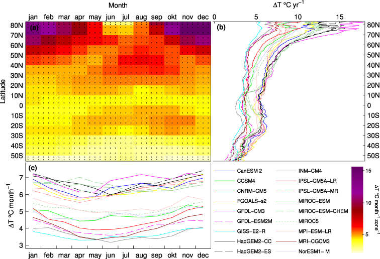
Figure 3. Seasonal–zonal land temperature patterns. (a) Simulated temperature change (2071–100 to 1961–90) (ΔT) from the 18 GCMs averaged over latitudinal bands of 10° and months. Colour indicates the 18 GCM average change, six dots implies that all GCMs agree on the sign of the change (all months and zones warms in all GCMs). (b) Annual ΔT as a function of latitude. (c) Monthly area weighed ΔT.
Download figure:
Standard imageAlthough there is agreement on the sign of the change of future ΔNEE between the simulations in the majority of month zones, there are still differences in the size of the change (figure 2(b)). Annually, the GCMs show large differences in ΔNEE between 40°N and 70°N, although most simulations predicts less uptake of carbon. Between 20°N and 30°S the simulations predicts both increased uptake, and increased release (or decreased sink) of carbon.
When considering the total monthly ΔNEE fluxes (figure 2(c)), the largest discrepancies between the simulations forced by different GCMs occur between July and October, likely as a result of differences in respiration associated with spread in summer and autumn temperatures (figure 3), as well as low agreement in the projections of precipitation change (figure S2 available at stacks.iop.org/ERL/7/044008/mmedia).
Even though the simulations show common patterns in terms of the sign of the change in NEE, its seasonality, and its zonal distribution, the discrepancies illustrated in figure 2 sum up to large differences over time, as shown in figure 4. The simulation forced by INM-CM4 results in the largest terrestrial carbon pool, 2232 Pg C, at year 2100 (2.27 Pg C yr−1 during 2006–100). GFDL-CM3 induces a source of carbon starting around year 2000, resulting in a total carbon terrestrial pool of 1862 Pg C at year 2100 (−0.97 Pg C yr−1 during 2006–100).
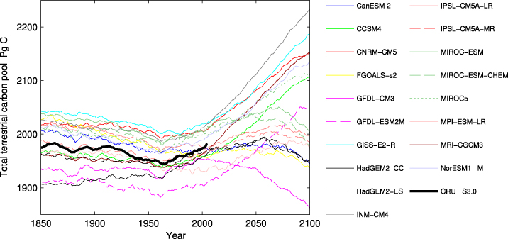
Figure 4. The total terrestrial carbon pool as simulated by LPJ-GUESS when forced by 18 GCMs and CRU TS3.0 historical data. A positive slope implies a negative NEE (sink of carbon), while a negative slope indicates a positive NEE (source of carbon).
Download figure:
Standard imageIn 10 of the 18 simulations the terrestrial biosphere switches from a sink to a source of CO2 before 2100 (negative slope), while 8 simulations result in a continued sink of carbon (positive slope) (figure 4). We find that the main explanatory factor underlying the spread in carbon uptake seen in figures 2 and 4 is the projected change in global land temperature (figure S3 available at stacks.iop.org/ERL/7/044008/mmedia). The global average land temperature for 2071–100 varies between 17.2 °C (GISS-E2-R) and 20.4 °C (GFDL-CM3) (an increase of 3.6–6.8 °C from the CRU 1961–90 temperature of 13.6 °C), explaining 93% of the variability in the simulated average 2071–100 NEE (figure S2 available at stacks.iop.org/ERL/7/044008/mmedia) (the land temperatures presented here exclude areas currently covered by ice sheets). The main underlying mechanisms are both a temperature-driven increase in evapotranspiration, drying-out soils and inhibiting plant production, and a positive effect of higher soil temperatures on decomposition, depleting soil carbon pools. The water balance-mediated mechanism may be most important in warm-climate ecosystems. There is evidence that interannual variations in atmospheric CO2 concentration over recent decades have been largely explained by episodes of drought in different regions (Zhao and Running 2010, Ahlström et al 2012b).
Spatially, the major patterns of change where a majority of the simulations (≥14/18) agree on the sign of the change are of a decreased uptake of carbon in North America and the western and central parts of Northern Eurasia (figure 5). The very high latitudes together with mountainous parts of South/Eastern Asia and parts of Brazil are major areas in which an increased uptake of carbon is projected by the majority of simulations. There is no or little agreement among simulations in the carbon balance response of the tropical rainforests.
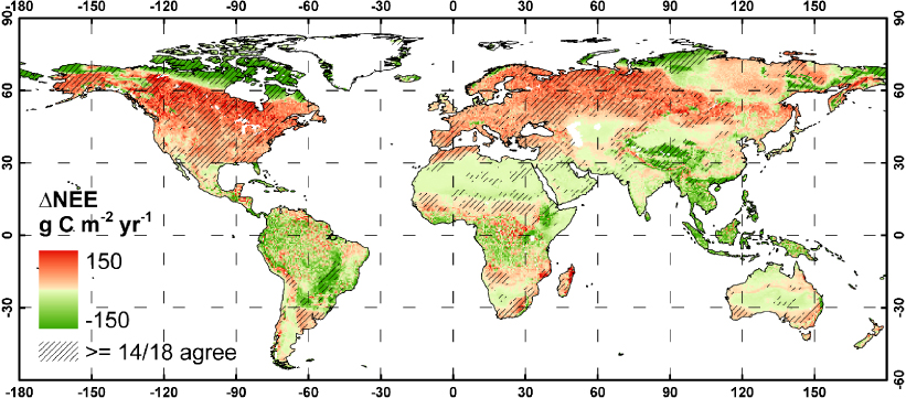
Figure 5. 18 simulation average ΔNEE and agreement between simulations. Colours indicate the 18 simulation average ΔNEE between 2071–100 and 1961–90. Areas where 14 or more of the 18 simulations agree on the sign of the change in NEE are highlighted with diagonal lines (filtered with a majority filter with window size of 3 × 3 gridcells, for clarity).
Download figure:
Standard image4. Discussion
Above we have shown that the LPJ-GUESS simulations forced with output from 18 different GCMs show agreement as well as disagreement in terms of temporal and spatial patterns of future carbon balance. All GCMs predict increased early spring temperatures resulting in a shift in extra-tropical phenology inducing an early spring uptake of carbon. Piao et al (2008) suggested that the uptake capacity of northern ecosystems may weaken if autumn temperatures warm at a faster rate than in spring. A majority of the GCMs (14/18) predicts a larger temperature increase in the autumn (August–October) compared to spring (March–May) (30°N–65°N). The warmer future autumn temperatures induce an average shift of the date when the ecosystem turns from a sink to a source—the zero-crossing date—(ecosystem respiration and fire > GPP) of −9 days between 1961–90 and 2071–100 (ranging from −15 to −2 days) in our results. However, as reported above, the date when the spring zero-crossing date—when the ecosystem turns from a net source to a sink—also occurs earlier (average =− 17 days, ranging from −21 to −9 days), leading to a longer period of net uptake in all 18 simulations. Instead the net loss seen in figure 2(b) is a result of a larger increase of release of carbon during autumn and winter compared to the increased sink seen during spring and summer (figure 2(c)). Similar to Qian et al (2010) we see an increased sink of carbon in the northern high latitudes (north of 65°) (not accounting for permafrost or wetland processes).
The fate of the tropics in terms of its future carbon balance has previously been found to be uncertain (e.g. Berthelot et al 2005, Friedlingstein et al 2006, Schaphoff et al 2006, Sitch et al 2008), our results show little agreement between simulations over months and latitudes (figure 2(a)) and annually across most of the tropics (figures 2(b) and 5).
The land use representation adopted in this study accounts for both deforestation associated with expansion of the area covered by cropland and grassland, and forest regrowth following abandonment of cropland and grassland. LPJ-GUESS includes an explicit representation of size structure and plant demographics and has demonstrated skill in reproducing succession and biomass accumulation following disturbance (Smith et al 2001, Hickler et al 2004). The importance of an adequate representation of demographics and size structure for accurate estimation of transient changes in carbon pools and fluxes for forest landscapes is increasingly recognized (e.g. Purves and Pacala 2008, Fisher et al 2010, Wolf et al 2011).
By applying different GCMs and ESMs to drive a single ecosystem model offline, as opposed to evaluating the outputs from the CMIP5 ESMs including a carbon cycle, we have focused on the uncertainties in future carbon balance arising from differences in the climate evolution simulated by different GCMs. Model intercomparison studies show that carbon balance changes projected by different DGVMs in response to the same forcing may also be substantial (Cramer et al 2001, Sitch et al 2008, Piao et al 2012). This aspect of uncertainty has not been considered by our study. However, LPJ-GUESS shows comparable behaviour and skill compared to other global ecosystem models. In a recent evaluation study encompassing ten DGVMs, Piao et al (2012) show, for example, that LPJ-GUESS falls in the middle of the range of other models in its prediction of present-day global GPP, in agreement with observation-based estimates, and exhibits comparable sensitivity to precipitation as suggested by upscaled ecosystem flux measurements. Our results demonstrate that interannual variation and geographic distribution of plant available water are key governing factors for land–atmosphere carbon exchange, echoing other recent studies (Zhao and Running 2010, Ahlström et al 2012b).
The spread of the change in the simulated total terrestrial carbon pool by nine of the ESMs applied in this study is about twice the spread of the LPJ-GUESS simulations using the climate outputs from the same nine ESM simulations (figure 6). Coupled ESMs generally amplify temperature increase and carbon balance changes, as a result of the positive feedback between temperature and the carbon cycle (Cox et al 2000, Friedlingstein et al 2006, Arneth et al 2010). However, the ESM simulations presented in figure 6 do not have an active carbon cycle feedback. The spread between the ESMs simulated terrestrial carbon cycle is induced by differences in simulated climate and differences between ecosystem models in the ESMs. The relative influence of the ecosystem model effect is difficult to separate from the climate in these simulations. Comparison of these ESM results with the results in this study applying the same sets of climate in a single vegetation model indicate that they are of a similar order of magnitude.
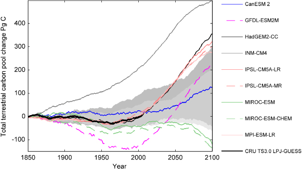
Figure 6. Change in total terrestrial carbon pool as simulated by nine CMIP5 ESMs. The graph shows cumulative net biospheric production (NBP), i.e. the change in the total terrestrial carbon pool, from nine of the CMIP5 ESMs applied in this study. The dark grey area shows the spread of the total terrestrial carbon pool from nine LPJ-GUESS simulations forced by interpolated (see section 2.2) original, uncorrected, climate fields from the nine ESMs presented above. The light grey area illustrates the spread of the LPJ-GUESS, bias corrected, simulations presented in this study for the same set of ESMs.
Download figure:
Standard imageAlthough the LPJ-GUESS simulations show agreement in the sign of the annual ΔNEE over much of the northern hemisphere, the large discrepancies in the magnitude of NEE change contribute significantly to the differences seen in accumulated carbon over time (figures 2 and 4). The discrepancies in accumulated carbon balance are a result of the large spread in northern hemisphere temperature (figure 3), as well as a considerable spread in temperature and low agreement among GCMs in the sign and magnitude of precipitation change in the tropics (figure S3 available at stacks.iop.org/ERL/7/044008/mmedia). Discrepancies in incoming shortwave radiation constitute an additional source of uncertainties. We find that the character and spatial patterns of GCM induced carbon balance uncertainties reported in previous studies (Berthelot et al 2005, Schaphoff et al 2006, Scholze et al 2006) are generally replicated by our model when forced by the chosen subset of CMIP5 output. In conclusion we argue that constraining the climate sensitivity, especially in the high latitudes, of the GCMs, in addition to narrowing tropical precipitation uncertainties, will contribute to narrowing the variability among projections of terrestrial carbon storage and release for the coming century.
Acknowledgments
This study was funded by the Swedish Foundation for Strategic Environment Research (Mistra) through the Mistra-SWECIA programme. The study is a contribution to the Lund University strategic research areas Modelling the Regional and Global Earth System (MERGE) and Biodiversity and Ecosystem Services in a Changing Climate (BECC). We acknowledge the World Climate Research Programme's Working Group on Coupled Modelling, which is responsible for CMIP, and we thank the climate modelling groups (listed in table 1 of this paper) for producing and making available their model output. For CMIP the US Department of Energy's Program for Climate Model Diagnosis and Intercomparison provides coordinating support and led development of software infrastructure in partnership with the Global Organization for Earth System Science Portals.