
Abstract
A method for defining and classifying heatwave events in the Euro-Mediterranean region is presented. The definition is based on the 95th centile of the local temperature probability density function, with additional criteria for spatial and temporal extension. The heatwave events are then classified into six classes by cluster analysis. The six heatwave patterns of Europe are described and compared to the existing literature. The most catastrophic extreme heatwaves (e.g. 2003 in Europe, 2010 in Russia) are shown to belong to one of these classes. It is then shown that the different classes are associated with different physical mechanisms. The effect of synoptic circulation and hydrological conditions are notably investigated. In particular, a drought appears to be a pre-requisite to heatwave occurrence in some clusters but not all.
Export citation and abstract BibTeX RIS
1. Introduction
Heatwaves have very serious consequences for society. Typical examples are the summer of 1995 in Chicago (Semenza et al 1996), or summers 1976 (Ellis et al 1980) and 2003 in Europe. This last event in particular was at the origin of 15 000 extra deaths (Hémon and Jougla 2003) in France and 70 000 in 12 European countries (WHO 2010). The remarkable intensity of this heatwave—the warmest over the last 500 yr over Europe according to Luterbacher et al (2004)—gave rise to a number of studies that highlighted its impacts on the economic and ecological systems, through reduction in productivity of natural and cultivated vegetation (Ciais et al 2005, COPA-COGECA 2003), lower energy supply and electricity restriction (Fink et al 2004), and an increase of air pollution (Vautard et al 2005).
Although such heatwaves are exceptional, several studies have shown that, associated with an increase of the temperature mean and variability in the context of global warming, these phenomena may become not only more frequent but also longer and more intense (Easterling et al 2000, Räisänen 2002, Klein Tank and Können 2003, Beniston 2004, Meehl and Tebaldi 2004, Schaer et al 2004, Klein Tank et al 2005, Della-Marta et al 2007).
Many physical mechanisms related to heatwaves have been studied. The key process is the presence of a persistent anticyclonic pattern over a high temperature area. In terms of 'weather regimes' (see Cassou et al 2005 and references therein), this pattern can be identified as an atmospheric blocking or—for Europe—as an Atlantic ridge putting western Europe under persistent southerly wind conditions. These atmospheric anomalies are the consequences of synoptic variability, but can also be influenced by large scale forcings. Cassou et al (2005) and Cassou (2008) investigated the influence of tropical oceans on weather patterns in the North Atlantic. They showed that the Madden–Julian Oscillation and anomalous tropical convection partially controls their distribution. Black and Sutton (2007) use a mechanism described in Rodwell and Hoskins (1996) to explain the teleconnection with the Indian Ocean. In some cases, the monsoon and anomalous sea surface temperature may create subsidence over the Mediterranean region and therefore inhibit convection. Hence precipitation and cloud cover are reduced on the mainland. Feudale and Shukla (2010) suggest that an increase of the sea surface temperature in the North Sea, the North Atlantic Ocean and the Mediterranean favors a barotropic response of the atmosphere that reduces the meridional gradient of temperature, consistent with a northward shift of the Inter-Tropical Convergence Zone (ITCZ) and of the descending branch of the Hadley cell. Land–atmosphere coupling, especially during drought, can amplify the temperature anomaly by increasing the sensible heat flux locally (Fischer et al 2007, Ferranti and Viterbo 2006). In Europe, the effect of drought can also be non-local (Zampieri et al 2009, Vautard et al 2007) with a cloudiness anomaly being advected from Southern Europe towards the North.
Most of these studies are either based on the only 2003 event, or they define heatwaves from temperature anomalies averaged over the whole European continent. In this letter, we want to take a more regional—event based—approach. One single heat wave event normally covers an area smaller than the continent; it is on the scale of the typical synoptic anomalies in the area, namely a few thousand kilometers. Distinguishing between different events, it may be asked which of the physical mechanisms above are preponderant to trigger or amplify a heat wave. A first step in that direction, therefore, is to establish an objective definition of a heatwave event and identify the typical heatwaves of Europe. We use a clustering approach to distinguish classes of heat wave events, following their geographical pattern. We also make a preliminary study on what the specific processes are that are associated with the different classes with respect to the synoptic situation and the hydrological pre-conditioning.
This letter is organized as follows. In section 2, we propose a definition of heatwave event and describe the clustering method. In section 3, we apply the clustering method to partition the set of previously defined heatwave events into typical classes. The classes are described and the atmospheric and hydrological conditions during and before the heatwave events are detailed. Section 4 discusses both the methodology and the results. Conclusions are given in section 5.
2. Methodology
2.1. Data source
We use a gridded version (E-OBS 3.0) of the European Climate Assessment & Data (ECA&D) (Klein Tank et al 2002) for continental surface temperature (mean, minimum and maximum) and precipitation (Haylock et al 2008). Hereafter, only maximum temperature and precipitation will be used for our study. The grid resolution is 0.5°× 0.5° and the data span from 1950 to 2009. Data observations were aggregated from several weather stations and gridded using an interpolation procedure combining spline interpolation and kriging. The interpolation smoothes the peak values inducing a 1.1 °C decrease of the median value of maximum temperature, if we consider an extreme event with a 10 yr return period (Haylock et al 2008). We select a domain over Europe and the Mediterranean region whose latitudinal and longitudinal boundaries are 30°N–70°N, 15°W–45°E, respectively.
The study period is 1950–2009 (60 yr) for which daily geopotential data from the National Centers for Environmental Prediction (NCEP) reanalysis (Kalnay et al 1996) were simultaneously available with 2.5° × 2.5° horizontal resolution available every 6 h. The reanalysis provides a complement for information about middle tropospheric conditions with the 500 mb geopotential height. For NCEP data the domain considered is extended to 30°–70°N, 70°W–45°E.
2.2. Data processing
2.2.1. Heatwave definition.
A range of weather-related and bioclimatic indices have been developed for heat wave definition, the relevance of which, regarding the impact on the natural and social system and on human health, have been reviewed in a number of reports and articles (WHO 2004, Laaidi et al 2004, Robinson 2001, Davis et al 2006). In this work, we use a simple definition based on temperature only: an extreme event is defined when the temperature exceeds a given threshold, and we impose additional constraints on the spatial and temporal extensions to avoid spurious intermittent and local events. Only summer is considered in this letter (June to August). In detail, a heatwave region is defined using the three following steps.
- (i)Temperature threshold: for each grid point, we consider a temperature anomaly with respect to the climatology (1950–2009) to be an extreme when its value exceeds the upper 95th centile of the local probability density function. The probability density function is computed for day D using the temperature data of the 60 yr climatology between D − 10 days and D + 10 days. For example to compute the 95th centile on 10 August at a given point, we use the local temperature values between 1 and 21 August of the 60 yr between 1950–2009.
- (ii)Spatial extension: taking a square of side L, there must be at least a fraction α of the surface where the temperature exceeds the upper 95th centile, using weights on the cosine of latitude. In this case, the central point of the square is retained as a heatwave point. This allows eliminating isolated 'hot' gridpoints. A sliding scan is performed with the square of side L over the whole domain. In the following, the results are shown for α = 0.6 and L = 3.75° in latitude and longitude. The sensitivity to the value of this parameters is investigated in section 4.
- (iii)Temporal extension: the above criteria are to be satisfied over at least four consecutive days. The temporal criterion is applied counting also adjacent regions. More precisely, when two heatwave squares overlap by more than 40% of their surface, they are retained as one single coherent event. This criterion thus allows us to smooth off some of the intermittency in the temperature signal, as well as to account for propagating phenomena.
2.2.2. Classification of heatwave patterns.
The above procedure identifies 78 heatwave events of 643 days total duration. The existence and characterization of typical heatwave patterns for the Euro-Mediterranean region are sought and a clustering technique is described hereafter for the classification.
Cluster analysis has been classically used in atmospheric sciences as a way to characterize mid-latitude weather. For a complete introduction to clustering methods see e.g. Tan et al (2006), for an extensive review of their use in atmospheric sciences, see Smyth et al (1999) and references therein. The main difficulty in the specific context of this letter is that only rare events are investigated, which by definition reduces the sample size for the clustering analysis. In this work, we have devised a clustering methodology that enhances the dissimilarity of the dataset. The clustering technique consists of three steps.
- (i)A pre-filtering of the data is performed. For each day belonging to one event, the temperature anomaly values at all grid points which are smaller than the 95th centile are set to zero.
- (ii)All pre-filtered daily maps belonging to one event are averaged producing 'event maps'.
- (iii)An agglomerative hierarchical clustering algorithm is applied to the event maps. At the initial step, each event map forms a cluster. The two 'nearest' clusters are then merged by pair into a new cluster. The distance between two clusters is measured using a metric defined below. This procedure is iterated until a stop criterion, defined hereafter, is met. The stop criterion sets the number of clusters.
All clustering methods require a metric definition d. Here, we use a pseudometric based on the anomaly correlation coefficient r, called also cosine similarity. First, we define a distance d' between any two maps p and q as:
with
where p and q refer to the maps which are matrices of size M by N along the longitudinal and latitudinal axes respectively, as in Cheng and Wallace (1993). The quantities pi,j and qi,j are the values of p and q at coordinates (i,j) along the longitudinal and latitudinal axes, respectively. The distance between two clusters C1 and C2 is then computed as the distance between their two farthest members, in other terms:

This definition of distance is particularly suited to distinguish between different spatial patterns of the temperature anomalies, while it is less sensitive to the amplitude of the temperature anomalies. d = 1 corresponds to orthogonal vectors, whereas d = 0 is for parallel vectors with a positive coefficient. Moreover d can be larger than 1 when vectors are anti-correlated.
The optimal number of clusters is found by plotting a dissimilarity index as a function of the number of clusters (figure 1). In any agglomerative clustering, the minimum distance can only continuously increase when the number of clusters decreases. Here, however, this index is defined as the minimum of the average inter-cluster distance (i.e. the distance of the two closest clusters). It can be seen in figure 1 that for seven clusters and more, the minimum inter-cluster distance reaches a minimum and remains almost constant. Increasing the number of clusters from six to seven means that one of the clusters is split into two clusters. The distance between these latter two clusters is very small because they remain very similar. In other terms, more partitions do not provide different patterns but merely place random borders within similar patterns. For much higher number of clusters (not shown), the dissimilarity index further decreases and reaches values that are indistinguishable from the dissimilarity of purely random partitions of the dataset.
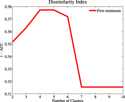
Figure 1. Dissimilarity index (minimum inter-cluster distance) as a function of the number of clusters.
Download figure:
Standard imageA cross validation procedure is used to check the stability of our classification. We eliminate 10 yr of the dataset to use as a verification period, and perform the clustering on the remaining 50 yr. Heat waves from the verification period are then associated to the six new clusters, according to the nearest distance. We compare the membership of the verification period episodes to the new 50 yr clusters to the membership of the full period clusters. This procedure is repeated six times for six sections of 10 yr over the 60 yr of record. A stability score is then computed by cluster: it is the ratio of the number of verification period heat waves that are correctly attributed over the total number of heat waves in the cluster.
These results are compared to a Monte Carlo test. The Monte Carlo test is constructed by proceeding as above, except that heat waves from the 10 yr verification period are associated to the 50 yr clusters in a purely random way, and the procedure is repeated 1000 times. From this, we estimate a PDF of the null hypothesis that the verification period heatwaves cannot be classified in the clusters obtained in the 50 yr period. The six clusters are significant to a 99% level. The IB and SC cluster are the most stable.
3. Heat waves clusters
3.1. Patterns description
Figure 2 shows the six typical heatwave patterns obtained after clustering. The patterns are represented by the average of temperature anomaly and 500 hPa geopotential height of all event maps of each cluster. The main geopotential anomaly structures are all significantly different from zero according to a two-sided t-test at the 99% level. The six patterns are labeled by a geographical acronym in the upper-left corner.

Figure 2. Six heatwave patterns obtained by a hierarchical clustering algorithm for the Euro-Mediterranean region: (a) 'Russian' cluster (RU), (b) 'Western Europe' cluster (WE), (c) 'Eastern Europe' cluster (EE), (d) 'Iberian' cluster (IB), (e) 'North Sea' cluster (NS) and (f) 'Scandinavian' cluster (SC). Daily maximum temperature anomalies are in color and expressed in deg K and isolines are the 500 hPa geopotential height anomaly.
Download figure:
Standard imageThe RU (Russia) cluster groups 128 days into 14 events. This class expands in the very north-eastern part of the domain over Russia between 35° and 45°E with a temperature anomaly up to 4 °C. It has a shape that is very similar to the one observed during the catastrophic Russian heatwave of summer 2010, although—notably—data from 2010 were not included in the analysis. The WE (Western Europe) cluster is centered mostly over France and has a magnitude of 5 °C. It includes 11 events for 82 days. The first half of August 2003 belongs to this cluster. The temperature anomaly pattern of the 2003 heatwave is very similar to the our WE pattern, if compared for instance with Schaer et al (2004). The temperature anomaly pattern displays a maximum North of the Alps and extends to the North and to the West with a slightly decreasing magnitude towards the Atlantic coast. The EE (Eastern Europe) cluster is approximately centered over Poland. Its magnitude is 4 °C with 23 events for a total of 182 days. It is relatively more spread out than the other clusters. A visual inspection of the different event maps shows events localized around the Baltic Sea and the Black Sea. The IB (Iberian) cluster is located over the Iberian Peninsula, with a second center over Turkey, along the same latitudinal band across the Mediterranean. It includes 75 hot days in nine heatwave events and displays the weakest temperature anomaly with maximum 3 °C. The NS (North Sea) cluster is the hottest, with a magnitude exceeding 6 °C above the mean. It includes 81 hot days in 11 events. The anomaly is centered over the North Sea and spans over Great Britain to the west, the Northern European coast and Eastern Scandinavia. Summer 1976 was very similar to the NS pattern when compared for instance with Fischer et al (2007). Finally, the SC (Scandinavian) cluster extends over most of the Scandinavian Peninsula with anomalies up to 6 °C. It includes 95 days in 10 events. The temporal succession of heatwave events is shown in figure 3. Notable recent events are present, for example the 2003 and 2006 West European heatwaves, or the North Sea event of 1976. Our methodology gives a heatwave duration of about one week for WE, EE, IB and NS whereas it is nine for RU and SC events.

Figure 3. Heatwave climatology in the Euro-Mediterranean region between 1950 and 2009 with attribution to the six heatwave clusters.
Download figure:
Standard imageFrom figure 2, we can see that all clusters have an anticyclonic anomaly in phase with the temperature anomaly. This is consistent with what is shown in the literature by many studies describing the climatology of heat waves. The European summer blocking high is visible in cluster WE as in Black et al (2004) or in Cassou et al (2005). The Ural blocking high is associated with the RU heatwave, as seen in 2010 (Barriopedro et al 2011). The only notable exception to the phase lock between the anticyclone and the temperature anomaly is the IB cluster. This cluster seems to be associated with a pattern similar to that of the EE cluster, with a high pressure over central Europe and a low over the Atlantic Ocean. In the IB cluster the peculiar position of the Atlantic low puts the Iberian Peninsula under southerly wind conditions. A similar condition can be seen over Turkey. It has already been observed that Iberian heatwaves tend to be triggered by warm advection from the Tropical Atlantic Ocean (Garcia-Herrera et al 2005). The connection with the Eastern Mediterranean is less obvious and could be due to a northward displacement of the subsiding part of the Hadley circulation.
3.2. Hydrological pre-conditioning
The importance of the soil moisture pre-conditioning in the context of heatwaves has been already emphasized by a number of studies (Huang and Van Den Dool 1992, D'Andrea et al 2006, Ferranti and Viterbo 2006, Seneviratne et al 2006, Fischer et al 2007), and drought conditions have often been shown to precede summer high amplitude temperature anomalies. As suggested by Vautard et al (2007) and Zampieri et al (2009) for the particular case of continental Europe, droughts in Southern Europe seem to precede heatwaves occurring in the most continental part of Europe.
In figure 4, the sensitivity of the temperature anomaly to the preceding hydrological conditions is thus analyzed for each cluster. Figure 4 shows the correlation between the rainfall occurrence anomaly between January and May, and the detrended summer maximum temperature anomaly at the heatwave location (the rainfall occurrence is the percentage of days between January and May for which daily accumulated rainfall exceeds 0.5 mm). We choose the frequency of rainy events as a proxy for soil moisture as in Vautard et al (2007) and Findell et al (2011). Considering that the correlation may not be latitudinally in phase as discussed in Vautard et al (2007), we plot in figure 4 the correlation as a function of different latitudinal bands. For WE and EE clusters, we can see a significant negative correlation between the rainfall occurrence anomaly and the summer maximum temperature anomaly between 40 and 45°N. This means that in Western and Eastern Europe, a positive temperature anomaly in summer (heatwave) is associated with a precipitation deficit in winter and spring in Southern Europe. This confirms, with a different approach and over a larger region, the results of Vautard et al (2007) and Zampieri et al (2009) which suggest that droughts in the south cause unusual low cloud cover which is then transported northward, reducing the convective instability and enhancing the anticyclonic conditions. However, this process is not as dominant for NS clusters for which the correlation is only marginally significant. In the case of IB, the heatwave is co-localized with the preceding rainfall deficit. The SC and RU clusters do not seem to be pre-conditioned by any rainfall occurrence anomaly.
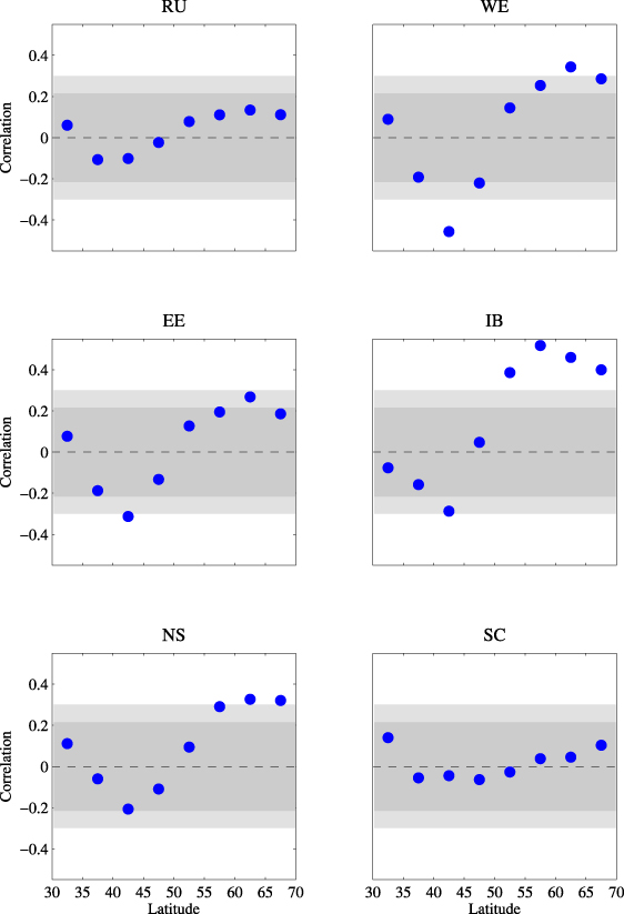
Figure 4. Correlation between the rainfall occurrence anomaly between January and May, and the detrended summer maximum temperature anomaly at the heatwave location (the rainfall occurrence is the percentage of days between January and May for which daily accumulated rainfall exceeds 0.5 mm). The dark gray shaded area indicates the 95% confidence interval bounds, whereas the light gray shaded area is for the 99% confidence interval bounds.
Download figure:
Standard imageThe correlations show a dipolar structure, with high correlation, significant in some clusters, with the northernmost latitudinal bands: these are probably due to a balance effect between northern and southern Europe. When rainfall decreases over Mediterranean Europe, it increases over northern Europe and vice versa. Such a phenomenon has been highlighted in previous studies and is very likely a manifestation of the North Atlantic Oscillation. Dai et al (1997) show evidence of an anti-correlation of the patterns of annual precipitation anomalies, between Scandinavian and continental Europe as well as the Mediterranean region. The existence of such dipoles is also illustrated in Uvo (2003) during DJFM (winter months). Uvo (2003) links the precipitation pattern to the different phases of NAO. In our case, the relation between heat wave and precipitation deficit in Southern Europe has a physically based explanation, as discussed in Vautard et al (2007) and Zampieri et al (2009). Conversely, we think that the positive correlation with precipitation excess in Northern Europe is purely statistical.
For the six hottest summers of clusters sensitive to Mediterranean drought (WE, EE, IB and NS), we show the rainfall structure over the entire domain stratified by clusters in figure 5. The pattern significance is assessed with a bootstrap method where samples of six different years are randomly picked over 1950–2009. We notice a shift in the water deficit along the longitude, fairly consistent with heat wave pattern location. It is especially striking for the EE cluster.

Figure 5. Composites of rainfall occurrence frequency anomaly from January to May, for the six hottest summers for WE, EE, IB and NS. The solid line represents the 90% confidence level.
Download figure:
Standard image4. Discussion
4.1. Classification method
There are three main parameters in our heatwave definition and classification method: the temperature anomaly threshold, the side of the scanning square L and the fraction α of the square area that must exceed the temperature threshold. In order to test the reproducibility of our results, we performed a sensitivity study where L and α have been modified. Modifying the threshold has a large impact on the results, but that amounts to changing the very definition of extreme events. The value of L has been varied between 2 and 7.5° of latitude and longitude. The difference in the total number of hot days selected was never larger than 40. Using a larger size L would not be appropriate because at this scale the number of sea points included in the square (that are excluded from the computation of the temperature threshold) would become very large. The parameter α does not modify the number of hot days for values ranging between 0.4 and 0.8.
The final list of 78 heat waves also compares well with other lists found in the literature. It includes seven of the ten hottest summers of Vautard et al (2007), which can be considered a good agreement given the difference of the domain and the definition of heatwave. A comparison with data from by Météo France on the 14 reported heat waves in France between 1950 and 2009 also shows good agreement (see http://comprendre.meteofrance.com/content/2010/5/23587-43.png). Eight of their ten episodes longer than four days are also present in our classification in either cluster WE or NS. The missing ones are absent from our list because they are classified as too short.
A similar study with minimum and mean temperature has also been performed. The hot day selections using mean temperature are very close to those using maximum temperature: it gives a total of 717 days, with a 83% overlap. The classification applied to minimum temperature is tantamount to a classification of hot nights. This gives a much smaller number of events, and a much smaller total number of hot nights (280). Most of the hot nights also correspond to a hot day (81%).
4.2. Heatwave classes
Varying the value of L does not change substantially the shape and the extent of the cluster patterns of figure 2. Indeed, the size and shape of the heatwave patterns is controlled by the size of the persistent anticyclone that controls in part the heatwave. As explained in many previous papers (e.g. Black et al 2004, Vautard et al 2007), heatwave events are primarily caused by the synoptic conditions. However, the pre-existing hydrological condition can influence the events by amplifying the temperature anomaly (Fischer et al 2007). We show in this study that the local or remote pre-conditioning by favorable hydrological conditions is not a universal feature for a heatwave, as shown for SC and RU clusters (figure 4).
In Koster et al (2004), it has been shown that the coupling between soil moisture and precipitation is active mainly in certain regions which they call 'hot spots'. Hot spots are located in transitional hydroclimatic regimes characterized by intermediate mean values and high variability of soil moisture as well as intermediate values and high variability of precipitation. In very humid areas, soil moisture tends to saturate and there is weak dependence between evapotranspiration and soil moisture. In a dry environment, tropospheric conditions are unfavorable to moist deep convection. Between these dry and moist extremes, there is potential for land-surface–atmosphere feedbacks.
In the context of heatwaves, it appears from our analysis that continental Europe shows the highest sensitivity to a pre-existing drought. Somewhat disappointing, Europe does not appear in the hot-spot map of Koster et al (2004), although the importance of soil moisture has been clearly highlighted in the many studies cited above. This probably has to do with the specific metric used by Koster et al (2004) and with the fact that their study is based on global models (for more details see the review by Seneviratne et al (2010)).
In the Scandinavian region (SC cluster), the land–vegetation system is rarely in water-limited conditions in summer. Moreover, its climate remains more dynamical than convective, being influenced by the polar front. The NS cluster shows a signal of sensitivity to soil moisture although it remains not significant. This is probably explainable with a sensitivity of the southern fringe of the region, located on the coast of the North Sea. The case of the RU cluster is somewhat different, for one might expect the temperate forestal areas of central Russia to satisfy the properties of the hot spots. However, it is possible that hydrology in those areas is influenced by more complex processes, like snow cover and snow melt, which make the proxy we used—rainfall anomaly occurrence—less pertinent. This class of heatwaves deserves further study, also in the light of the 2010 event.
5. Summary and conclusion
A heat wave classification over the period 1950–2009 in the Euro-Mediterranean region has been carried out by means of a gridded observation dataset. Our definition of heat waves is consistent with official data and literature, including all the major events of the last decade. Despite the difficulty inherent in the limited data available, the classification algorithm partitions the 78 heatwave events into six classes: Russian, West European, East European, Iberian, Scandinavian patterns and one last pattern centered over the North Sea. These are the typical heatwaves of Europe.
High temperatures are co-localized with fair weather and a high-pressure system. This brings an increase of radiative forcing and thus sensible heat flux and temperature rise. Heatwaves in the WE and EE clusters are preceded by rainfall deficit in Southern Europe, as in Vautard et al (2007). This is not the case for the northernmost clusters (SC and RU). The Iberian pattern is caused by warm air advection from the south and is preceded by a drought at the same location as the heatwave.
Acknowledgments
This work is a contribution to the MORCE-MED project funded by the GIS (Groupement d'Intérêt Scientifique) 'Climat, Environnement et Société'. This work also contributes to the HyMeX program (HYdrological cycle in The Mediterranean EXperiment; Drobinski et al (2009, 2010)) through INSU-MISTRALS support. The authors are grateful to A Ducharne and R Vautard for fruitful discussions.