


Abstract
Recent observations indicate that two cryospheric components, namely the Antarctic sea ice and ice shelf over the Southern Ocean, have been changing over the decades. Here we analyze results from an ocean–sea ice–ice shelf model to examine variability in the Antarctic sea-ice extent and ice-shelf basal melting. The model reproduces seasonal and interannual variability in the Antarctic sea-ice extent and demonstrates that summertime ice-shelf basal melting is closely anti-correlated with the sea-ice extent anomaly. For example, the unprecedented minimum of the Antarctic sea-ice extent in the 2016 spring was accompanied by a substantial increase in the Antarctic ice-shelf melting in the model. Detailed analysis of Antarctic coastal water masses flowing into the ice-shelf cavities illustrates the physical linkage in the strong anti-correlation. This study suggests that the Antarctic summer sea-ice extent in the regions where the sea-ice edge approaches the Antarctic coastline can be a proxy for Antarctic coastal water masses and subsequent ice-shelf basal melting.
Export citation and abstract BibTeX RIS

Original content from this work may be used under the terms of the Creative Commons Attribution 4.0 license. Any further distribution of this work must maintain attribution to the author(s) and the title of the work, journal citation and DOI.
1. Introduction
The Southern Ocean is the only ocean that directly connects three oceans: the Atlantic, Indian, and Pacific Oceans. Thus, the Southern Ocean plays a crucial role in the formation and changes in the global ocean and climate. There are two cryospheric components whose processes affect the Southern Ocean water masses' formation and changes: Antarctic sea ice and ice sheet. These two components are strongly linked to freshwater fluxes on the Southern Ocean surface. Sea ice is formed from seawater when the ocean surface is strongly cooled in autumn and winter, and it melts in summer, contributing to the separation and redistribution of salt and freshwater (Pellichero et al 2018). Dense Shelf Water (DSW), a precursor of Antarctic Bottom Water, is formed along the Antarctic coastal margins (in particular, coastal polynyas) when salt is rejected into seawater during intensive sea-ice formation (Morales Maqueda et al 2004). In summer, melting of sea ice causes freshwater input to the ocean surface, contributing to the formation of summertime surface stratification. The Antarctic ice sheet is a gigantic ice block on the Antarctic continent, and the termini protrude into the Southern Ocean in numerous places, forming Antarctic ice shelves. The ice shelves are responsible for the Antarctic ice sheet's ablation processes through basal melting and iceberg calving. Melting of the Antarctic ice-shelf bases and icebergs is another source of freshwater fluxes for the Southern Ocean. Recent satellite and historical hydrographic observations suggest that the Southern Ocean and the ambient cryospheric components have changed over the decades (Parkinson 2019, Rignot et al 2019). These changes may result in wide-ranging ramifications not only in the Southern Ocean but also for the global ocean (Convey et al 2009, Turner et al 2009).
With the advent of modern satellite remote sensing observations, sea-ice concentration and extent in both polar regions can be accurately monitored daily. The Southern Ocean has the most seasonally variable sea-ice cover on the Earth, with a spatial extent ranging from 3 × 10⁶ km2 in summer to 19 × 106 km2 in winter (figure 1(b)). The variability of the Antarctic sea ice over the last four decades is fascinating (Parkinson 2019). The Antarctic sea-ice extent had gradually expanded from the late 1970s to 2015 (Parkinson and Cavalieri 2012, Comiso et al 2017, de Santis et al 2017). However, in the 2016 spring, the Antarctic sea-ice extent anomaly recorded the minimum in recent decades and continues to be in the negative phase in the last few years (Reid et al 2017, Stuecker et al 2017, Turner et al 2017, Kusahara et al 2018). In contrast to the spatially and temporally high-resolution sea-ice observation, the ablation processes at the Antarctic ice shelves (i.e. ice-shelf basal melting and iceberg formation) have only recently been estimated from a combination of satellite-based ice flow observations and snow accumulation modeling, illustrating that ice-shelf basal melting is the dominant process for the Antarctic ice sheet mass balance (Depoorter et al 2013, Rignot et al 2013). The commonly-used estimates of ice-shelf basal melting represent a climatological value or mean value averaged over a relatively short period of the analyses. The temporal variability of Antarctic ice-shelf basal melting has become an important research topic in Antarctic and Southern Ocean studies (Jenkins et al 2018, Adusumilli et al 2020).
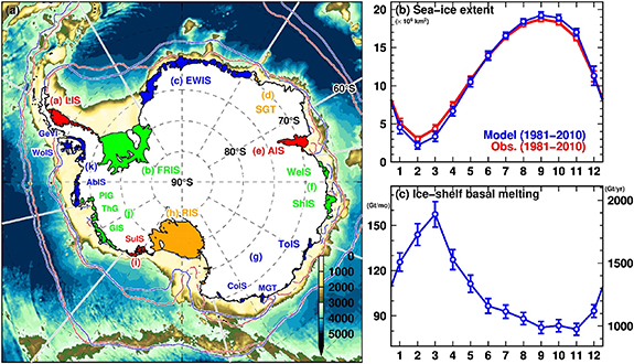
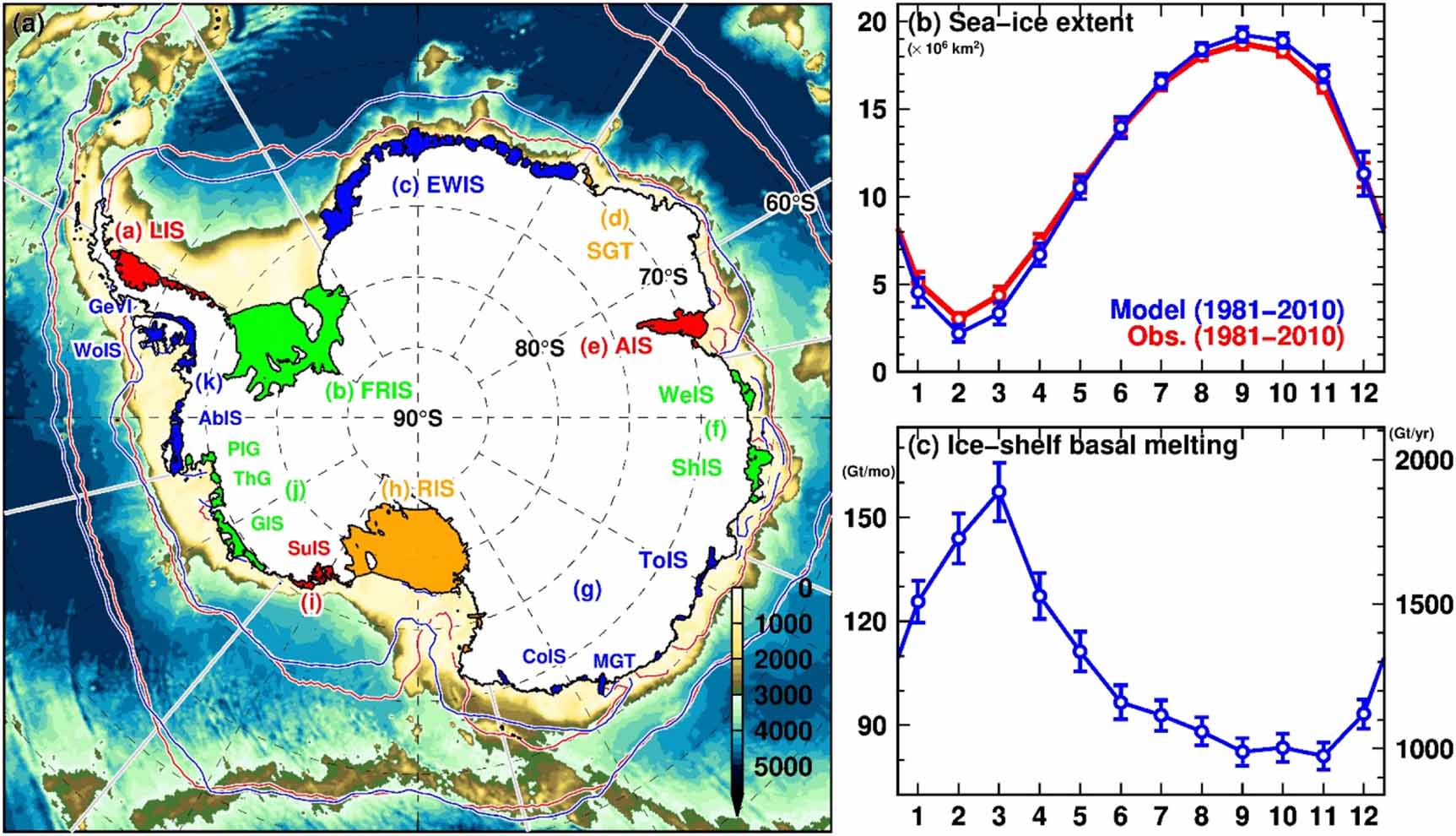
Figure 1. (a) Model bottom topography and (b), (c) seasonal cycles of the Antarctic sea-ice exetent and ice-shelf basal melting. Eleven groups of ice shelves (labels (a)–(k)) are shown by different colors (red, green, blue, and orange). In the right panels, red and blue colors indicate results from the satellite observation and the model. In panel (a), the observed and modeled sea-ice edges in winter (July–September) and summer (January–March) are overlaid with red and blue curves, respectively. The period for calculating the climatology in this plot is 1981–2010. Gray lines are boundaries for calculating regional sea-ice variability. Major ice shelves/glaciers are shown in the same grouping colors: Larsen Ice Shelves (LIS), Filchner–Ronne Ice Shelf (FRIS), Eastern Weddell Ice Shelves (EWIS), Shirase Glacier Tongue (SGT), Amery Ice Shelf (AIS), West Ice Shelf (WeIS), Shackleton Ice Shelf (ShIS), Totten Ice Shelf (ToIS), Mertz Glacier Tongue (MGT), Cook Ice Shelf (CoIS), Ross Ice Shelf (RIS), Sulzberger Ice Shelf (SuIS), Getz Ice Shelf (GIS), Thwaites Glacier (ThG), Pine Island Glacier (PIG), Abbot Ice Shelf (AbIS), Wordie Ice Shelf (WoIS), and George VI Ice Shelf (GeVI).
Download figure:
Standard image High-resolution imageJacobs et al (1992) introduced three modes to explain Antarctic ice-shelf basal melting. Three water masses of DSW, Circumpolar Deep Water (CDW), and Antarctic Surface Water (AASW) play roles in the three basal melting modes. Although DSW is a cold water mass, it is responsible for Mode-1 melting because the freezing point of seawater decreases with depth/pressure. CDW is a portion of the Antarctic Circumpolar Current at intermediate depths and is characterized by high temperature and high salinity. Therefore, a part of the CDW that intrudes onto the continental shelf regions across shelf breaks can melt ice-shelf bases very effectively (Mode-2). In summer, AASW is formed by a combination of sea-ice meltwater and surface heating during the sea ice‐free period. AASW is a relatively warm water mass and can serve as an effective heat source for ice-shelf basal melting (Mode-3) when AASW is transported into ice-shelf cavities. The variability in the coastal water masses flowing into ice-shelf cavities controls the spatiotemporal variability in the Antarctic ice-shelf basal melting (Kusahara 2020). Sea-ice-related processes play a role in the water mass formation: sea-ice formation and melting along the Antarctic coastal margins are responsible for the DSW formation in winter and the summertime surface water formation, respectively.
This study performed a numerical simulation of an ocean–sea ice–ice shelf model that can reasonably reproduce the Antarctic sea-ice variability in recent decades to investigate the relationships between the Antarctic sea-ice extent, coastal water masses, and ice-shelf basal melting. This study focuses on the summer season because ice-shelf melting is the most pronounced in a year, and the variability is interlocked with the sea-ice variability through the coastal water masses' variability in many places (as shown below). In section 2, we examine the seasonal and interannual variability in the Antarctic sea-ice exetent and ice-shelf basal melting in the model. The details of the model configuration and experiments are provided in appendix A (in the supplemental material (available online at stacks.iop.org/ERL/16/074042/mmedia)). In section 3, we analyzed in detail the temporal variability in the Antarctic coastal water masses flowing into the ice-shelf cavities to elucidate the linkage between the two cryospheric components. In section 4, we summarize our findings and contrast them with the literature in terms of the ocean‒sea ice–ice shelf interactions over the Southern Ocean.
2. Sea-ice extent and ice-shelf basal melting: circumpolar and regional perspectives
This study used results from an ocean–sea ice–ice shelf model in a realistic configuration for the circumpolar Southern Ocean (figure 1(a)) for the period 1979‒2018 (appendix A in the supplementary material). In this section, we show seasonal and interannual variations in the Antarctic sea-ice extent and ice-shelf basal melting in the model, including validations with the available observations. Afterwards, we examine the relationships between the two cryospheric components from the circumpolar-scale and regional-scale perspectives. In the next section, we present the results of a detailed analysis of the Antarctic coastal water masses that connect the two components.
This study utilizes 30 year averages for the period 1981–2010 to investigate the seasonal variation of variables, such as sea-ice extent/concentration and ice-shelf basal melting. We used the sea-ice concentration by the NASA Team algorithm as the observed sea ice (Cavalieri et al 1984, Swift and Cavalieri 1985). The numerical model realistically reproduces the seasonal variation in the Antarctic sea-ice extent (figure 1(b)). However, the model tends to underestimate the total sea-ice extent in summer and overestimate it in winter. Underestimation of the summertime sea-ice extent originates from that along the East Antarctic coast (figure 1(a)). The interannual variability in the total sea-ice extent is the largest in December and January (see the error bars in figure 1(b)).
The seasonal variation in Antarctic ice-shelf basal melting shows a maximum in summer and minimum in winter, which is almost the opposite seasonal cycle of the sea-ice extent (figures 1(b) and (c)). The maximum of the ice-shelf basal melting in the model is approximately 1900 Gt yr−1 (in the equivalent annual melt amount) in March, and the minimum with approximately 1000 Gt yr−1 from September to November. The seasonality of the ice-shelf basal melting in this model is consistent with a previous modeling study (Dinniman et al 2015). The annual mean of the total ice-shelf basal melting in the model for the period 1981–2010 is 1284 Gt yr−1, roughly consistent with the satellite observation-based estimates of Depoorter et al (2013) and Rignot et al (2013) of 1454–1500 Gt yr−1. However, the model has regional biases (appendix B): the model underestimates the basal melt amount in ice shelf group (j) (GIS/ThG/PIG) in the Amundsen Sea due to the regional cold biases (figure B3), and overestimates that in ice shelf group (c) (EWIS) in the Atlantic sector due to exaggerated warm water intrusions (figures B2 and B3). Non-negligible regional biases due to overestimating the warm waters are also found in the ice shelf group (h) (RIS) and (i) (SuIS) in the Ross Sea. Nevertheless, the opposite regional model biases compensate for each other, resulting in the agreement in the total basal melt amount of the Antarctic ice shelves.
The red and orange curves in figure 2(a) indicate the monthly sea-ice extent anomalies in the model and the observation for the period 1979–2018. The monthly sea-ice extent anomaly was calculated by subtracting the climatological monthly sea-ice extent (figure 1(b)) from the monthly sea-ice exetent each month. The similarity in the two time series confirms that the model can reproduce the temporal variability in the total Antarctic sea-ice extent (figure 2(a)) as well as the seasonal cycle (figure 1(b)). In particular, the model can represent the long-term trend in the total sea-ice extent anomaly for the period from the late 1970s to 2015 and a rapid decline from positive to negative in the 2016 spring. The model's ability gives us some confidence to investigate the relationship of ice-shelf basal melting and Antarctic coastal water masses with the sea-ice fields (see also Kusahara et al (2017, 2018, 2019) for the sea-ice model performance).

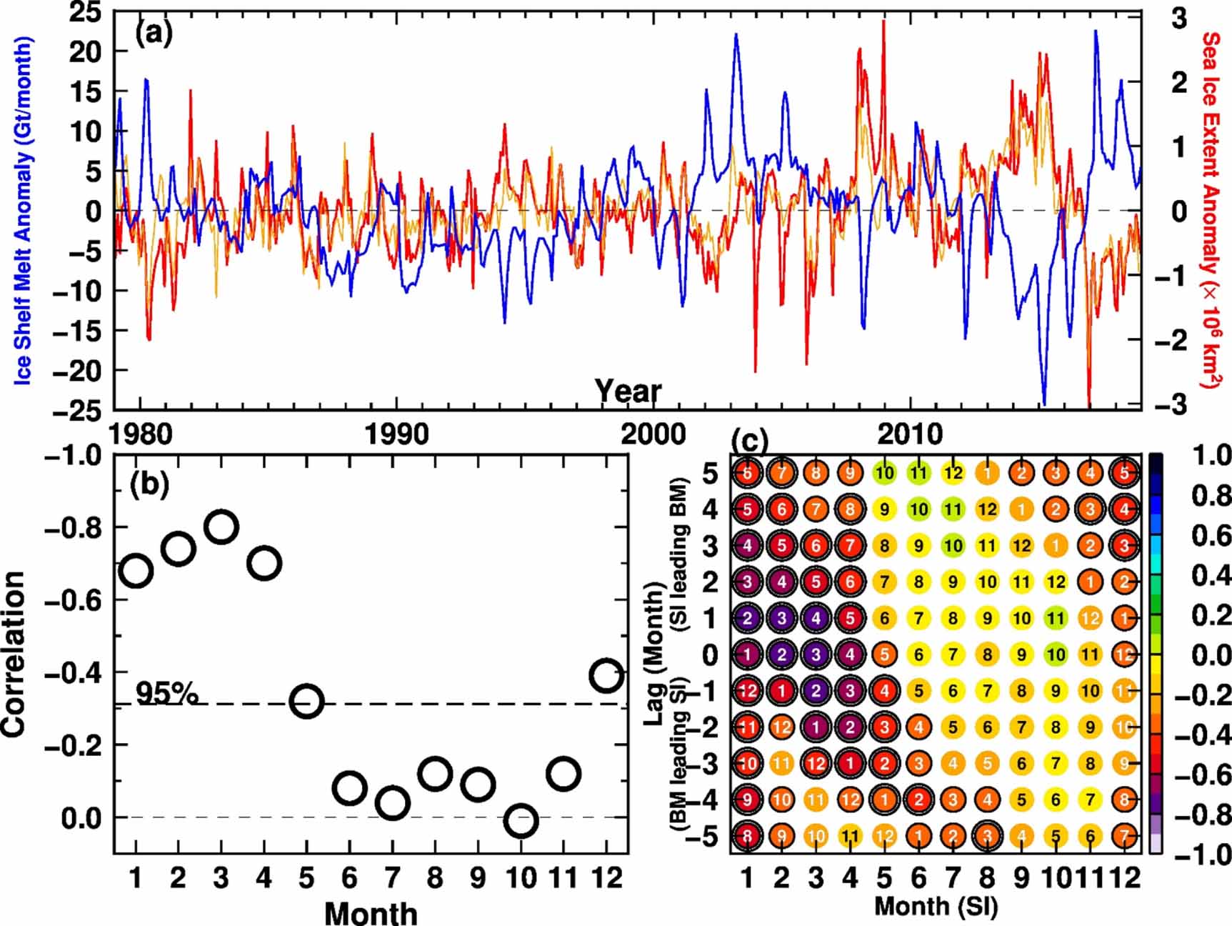
Figure 2. (a) Time series of monthly SI sea-ice extent anomalies (red: model and orange: observation) and ice-shelf basal melting anomaly (blue), (b) the monthly correlation coefficients between the two, and (c) the lag correlation coefficients. In panel (c), single and double black circles represent exceeding 95% and 99% significant levels, respectively. White and black numbers indicate month of the ice-shelf in the lag correlation analysis.
Download figure:
Standard image High-resolution imageThe monthly anomaly time series of the Antarctic ice-shelf basal melting was calculated similarly to the sea-ice extent anomaly calculation (blue curve in figure 2). Interestingly, there is a significant anti-correlated relationship between the total sea-ice extent anomaly and the ice-shelf melting anomaly, with statistically significant correlation coefficients (r = −0.46 for the raw anomaly time series and r = −0.63 for the 13 month running mean time series). When the Antarctic total sea-ice extent shifted to a negative phase in late 2016, the ice-shelf basal melting anomaly shifted from a negative to a positive anomaly. The negatively-correlated relationship between the two time series is confirmed throughout the analyzed period (1979–2018).
To further examine the seasonality of the anti-correlated relationship, we calculated the simultaneous and lag correlation coefficients between the two anomalies for each month (figures 2(b) and (c)). The statistically significant negative correlation coefficients are extensively found in summer at zero-time lag and also in a phase when the sea-ice variability leads the ice-shelf basal melting (figure 2(c)). Looking at the zero-lag correlations (figure 2(b)), there are statistically significant correlation coefficients in the summer months from December to May, with the highest magnitude of the coefficients from January to April (>0.6 in magnitude). This result demonstrates the sea-ice extent and ice-shelf basal melting in the model covary in summer. It should be noted that significant lag correlation coefficients in an autumn regime (April‒June) where ice-shelf basal melting seems to precede the sea-ice variability are pseudo-signals caused by long durations of the sea-ice and the ice-shelf basal melting variability over several months (figure S3). High autocorrelation coefficients of the sea-ice extent variability in summer of several months (figure S3(a)) mean that the summer sea-ice conditions affect the subsequent autumn sea-ice fields to some extent. The autocorrelation length of ice-shelf basal melting is longer than that of sea ice, lasting more than half a year (figure S3(b)). These long durations of the sea-ice and the ice-shelf basal melting variability create the significant correlations in the autumn regime. We confirmed from a numerical experiment without ice-shelf melting (in a similar model configuration) that ice-shelf melting has a very minor impact on the Antarctic sea-ice variability (Kusahara et al 2017).
Next, we apply the same correlation analyses to the regional sea-ice extent and ice-shelf basal melting to examine regional differences (figures S1 and S2). In this study, Antarctic ice shelves were divided into 11 groups based on their geographical locations (labeled (a)–(k) in figure 1(a)). Nine sectors were defined to calculate the regional sea-ice extent (see gray lines in figure 1(a) for the boundaries). Figures S1(a)–(c) show the monthly correlation coefficients between the regional ice-shelf basal melting and the adjacent sector's sea-ice extent. Except for ice shelf group (i) (SuIS), all the ice shelf groups show anti-correlated relationships between sea-ice extent and ice-shelf basal melting in summer. In particular, statistically significant negative correlations (|r| > 0.6) are obtained for ice shelf groups (c) (EWIS), (d) (SGT), (e) (AIS), (f) (WeIS/ShIS), (g) (ToIS/MGT/CoIS), (j) (GIS/ThG/PIC), and (k) (AbIS/WoIS/GeVI) during January–April. Lag correlations coefficients (figure S2) highlights the regional nature of relationship between the sea-ice extent and ice-shelf basal melting. The significant negative correlation coefficients at zero-lag or the sea-ice leading phase (upper side of each panel in figure S2 are found at the ice shelves where sea ice largely retreats in summer (i.e. the regional sea-ice edge is very close to the Antarctic coastline or ice-shelf front (figure 1(a))). Ice shelves where the summer sea-ice edge is outside of the neighboring continental shelf (ice shelf groups (a) (LIS), (b) (FRIS), and (i) (SuIS)) show different patterns in the lag correlation analyses. As shown in the next section, the sea-ice extent variability in these regions is weakly related to variability in the coastal water masses and the ice-shelf basal melting.
3. Antarctic coastal water masses
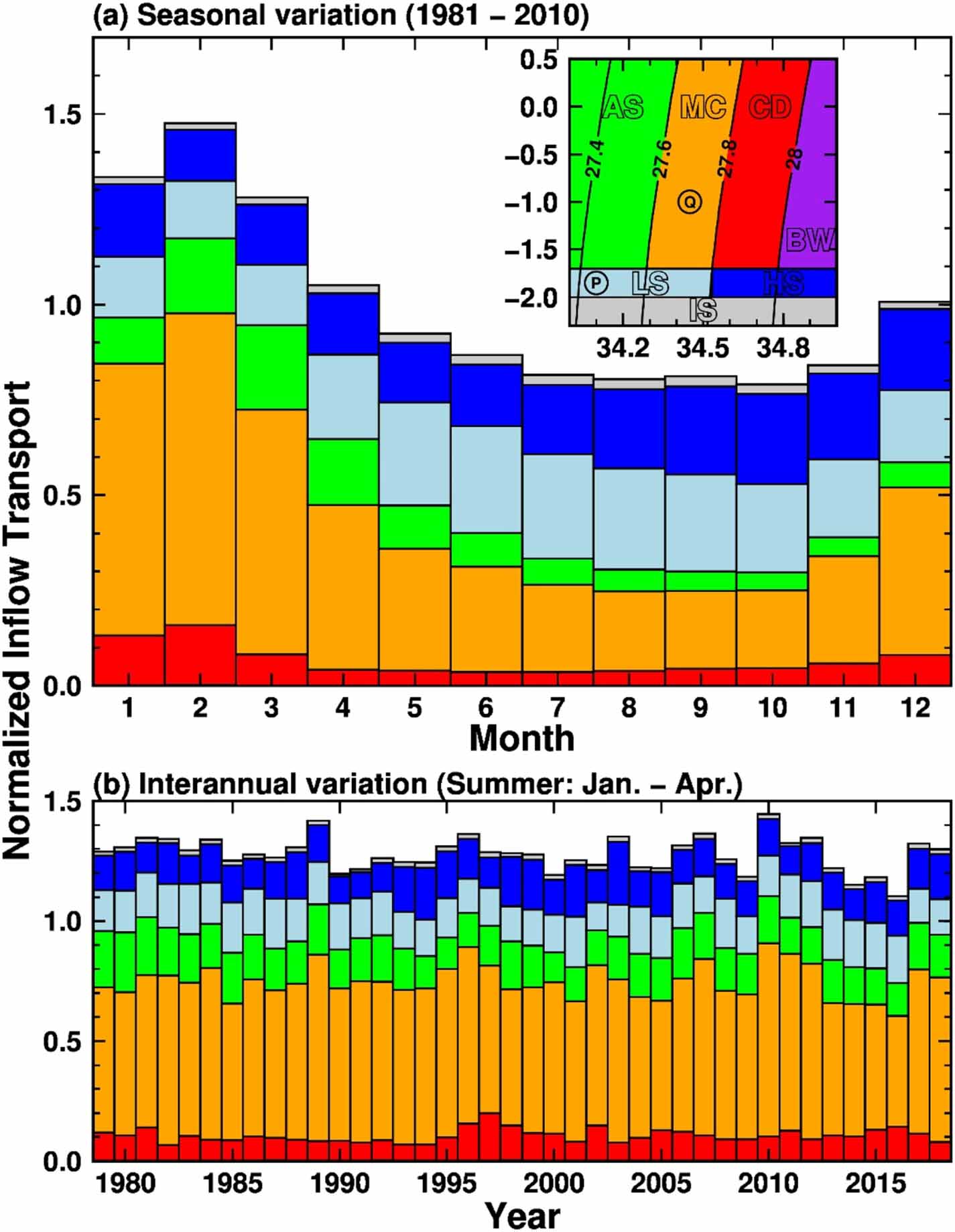
Here, we examine in detail the variability of Antarctic coastal water masses that connect the two cryospheric components of the Antarctic sea-ice extent and ice-shelf basal melting. To begin with, we examine the Antarctic coastal water masses flowing into the ice-shelf cavities (exactly across the ice-shelf fronts in the model) to identify the ocean heat source for ice-shelf melting in the model. Seven coastal water masses were defined based on the ocean temperature (θ), salinity, and potential density anomaly (σ0). The classifications are displayed in the T–S diagram in figure 3(a). Note that the classification of the coastal water masses is empirical and slightly unconventional. However, it is convenient to evaluate the water masses all over the Antarctic coastal regions with a single framework. High salinity shelf water (labeled 'HS' in the T–S diagram in figure 3) was introduced as DSW for Mode-1 melting. The lower-salinity variety was defined as low salinity shelf water ('LS'). The two water masses are cold water (−2.0 °C ⩽ θ < −1.7 °C). The salinity boundary between the LS and HS was set to 34.534 psu, which is the salinity on the potential density surface of 27.8 kg m−3 at −1.7 °C. With this LS definition, LS corresponds to low-salinity DSW or cold, less dense water originated from sea-ice melting. Four water masses with a relatively high temperature (θ ⩾ −1.7 °C) were defined using the potential density anomaly. The densest water is labeled BW (bottom water), and it is denser than the potential density of 28.0 kg m−3. CDW for Mode-2 melting was defined with a density range 27.8 kg m−3 ⩽ σ0 < 28.0 kg m−3 (labeled 'CD'), while AASW for Mode-3 melting was defined with the least dense water (σ0 < 27.6 kg m−3, labeled with 'AS'). The intermediate-density water between CD and AS was classified as modified circumpolar deep water ('MC'). Water colder than −2 °C was defined as Ice Shelf Water ('IS'). The inflow transports of BW and IS into the ice shelf cavities are very small. The remaining five water masses (CD, MC, AS, LS, and HS) are the primary heat sources for the Antarctic ice-shelf basal melting in this model. Hereafter, we examine the temporal variability in the five coastal water masses and the relationships with the sea-ice and ice-shelf melting variations.
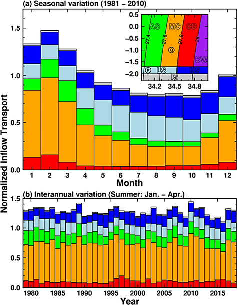
Figure 3. Seasonal and interannual variations of the Antarctic coastal water masses' inflow transport into the ice-shelf cavities. The T–S diagram in panel (a) shows the water masses' definitions used in this study (see the main text for the water mass classification). The climatology for the period 1981–2010 is used for the seasonal variation in panel (a). The summertime averages during January–April are shown in panel (b). All the water masses' transport is normalized with the climatology of the annual-mean total inflow transport.
Download figure:
Standard image High-resolution imageFigure 3(a) shows the seasonal variation of the coastal water masses' transport into the Antarctic ice shelf cavities to explain the seasonality in the ice-shelf basal melting (figure 1(b)). The monthly inflow transports of the coastal water masses were normalized by the average annual-mean of the total inflow transport into the cavities. The 1981‒2010 average was used for the normalization. The normalization allows us to highlight the regional differences (figure B2). For the Antarctic ice shelves as a whole (figure 3(a)), there are large seasonalities in the total transport and component ratio of the coastal water masses flowing into the cavities. The inflow transports of the relatively warm water masses of CD, MC, and AS peak in summer, and they contribute considerably to the total transport amount. On the other hand, the inflow transports of the cold water masses of HS and LS peaks in winter when the total transport reaches the minimum. These seasonal variations in the warm and cold waters control the seasonality in heat transport into the cavities and the subsequent ice-shelf basal melting. It should be noted that the inflow transport of AS is seen even in winter in figures 3(a) and B2, but this water mass is not warm surface water originating from sea-ice meltwater and surface heating. Water from a mixture of LS and MC (see the points P and Q in the T–S diagram in figure 3) is also categorized as AS in this analysis.
Figure 3(b) shows the interannual variation of the summertime Antarctic water masses' transports into the Antarctic ice shelf cavities for the period 1979–2018. As seen in the time series, there is a pronounced year-to-year variability in both the total transport and the component ratio of the coastal water masses. To quantify the summertime relationships among the variabilities in the sea-ice extent, ice-shelf basal melting, and Antarctic coastal water masses, we calculated correlation coefficients between the two variables among them for regional and circumpolar perspectives (figure 4).

Figure 4. Correlation coefficients between the variables (SI: sea-ice extent, BM: ice-shelf basal melting, and the five Antarctic coastal water masses' inflow transports) in the summer season (from January to April). See the T–S diagram in figure 3(a) for the water mass definition. Red and blue lines indicate positive and negative correlations, respectively. Numbers near the lines connecting two variables represent the correlation coefficient between the two. Thick and medium-thick lines indicate exceeding 99% and 95% significant levels, respectively. Missing lines between two neighboring variables indicate that the length of either or both variables is less than 50% of the total length of the analysis period.
Download figure:
Standard image High-resolution image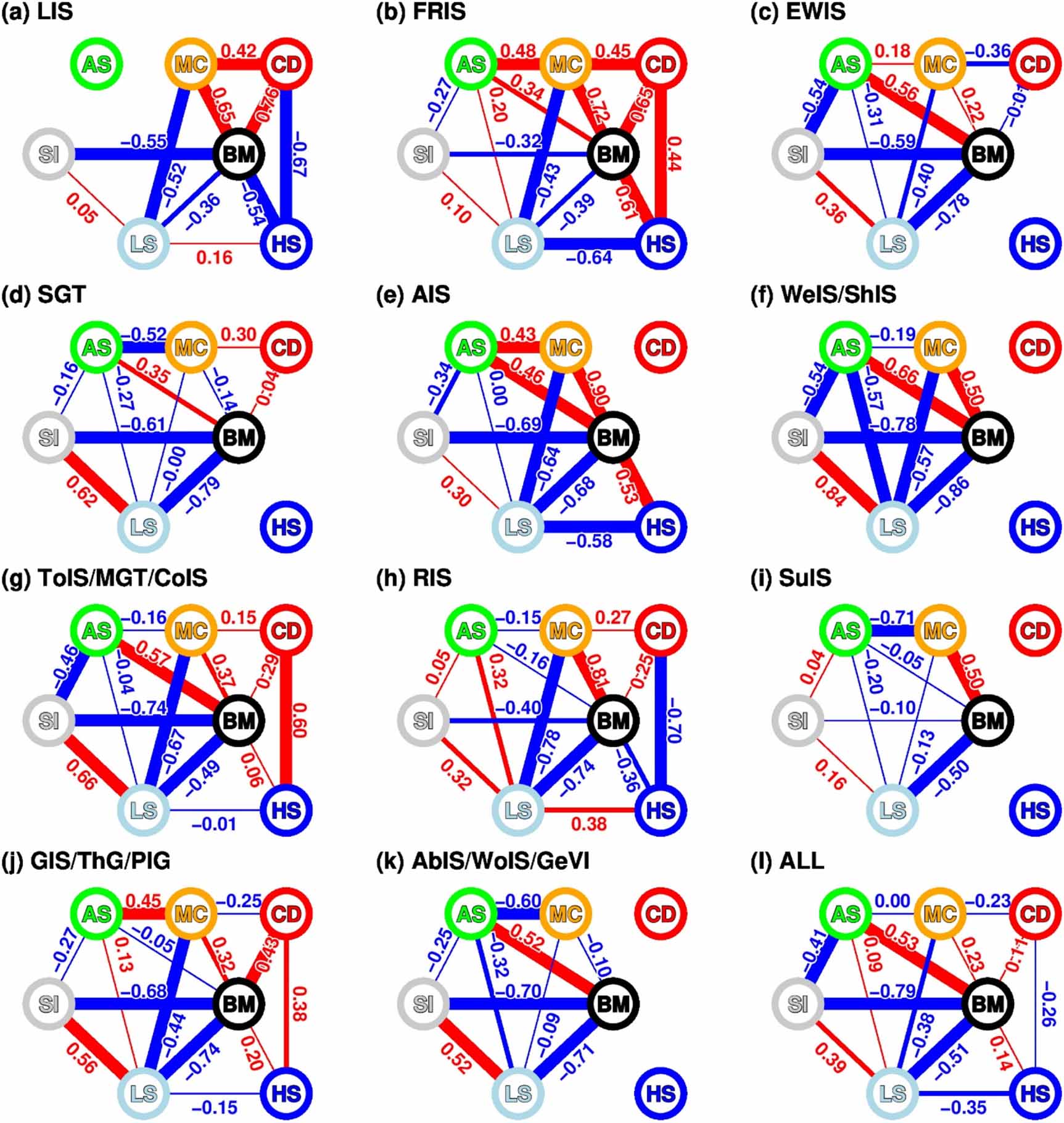
The comprehensive correlation analyses for the ocean-cryosphere variables reveal the regional similarity and difference in the variables' relationships. Here, we first focus on the relationship of the regional ice-shelf basal melting with the five coastal water masses (AS, MC, CD, LS, and HS, see T‒S diagram in figure 3(a)). For all ice shelves (figures 4(a)‒(k)), ice-shelf basal melting has a statistically significant positive correlation with at least one of the three warm water masses (AS, MC, CD), confirming that these water masses are heat sources for the Antarctic ice-shelf basal melting in summer. The strongest positive correlation coefficients between ice-shelf basal melting and AS are found in ice shelves (c) (EWIS), (e) (AIS), (f) (WeIS/ShIS), (g) (ToIS/MGT/CoIS), and (k) (AbIS/WoIS/GeVI). We next show the relationship with the relatively cold water masses (LS and HS). The regional correlation coefficients between BM and LS show statistically negative for all ice shelves, indicating that the LS inflow suppresses ice-shelf basal melting. The correlation coefficients between BM and HS are negative at ice shelves (a) (LIS) and (h) (RIS), while they are positive at ice shelves (b) (FRIS) and (e) (AIS) (the correlation coefficients for the other ice shelves are insignificant). In this model, warm waters (CD and MC) account for approximately half of the summertime inflow in the former ice shelves (a) (LIS) and (h) (RIS). Under these conditions, an increase in the percentage of HS leads to a decrease in the percentage of the warm waters, having the effect of suppressing the ice-shelf basal melting as well as LS. On the other hand, at the latter ice shelves ((b) and (e)), where cold water masses dominate the total inflow, the inflow of HS becomes a heat source for ice-shelf basal melting. These ice shelves' drafts are relatively deep, so that HS, which is a dense cold water mass with a near-surface freezing point, can also be an effective heat source for ice-shelf basal melting.
Next, we examine the relationship between the two surface water masses (AS and LS) and the sea-ice extent (SI). Our previous modeling study (Kusahara et al 2019) demonstrated that interannual variability in the summertime Antarctic sea-ice extent is regulated by a combination of wind stresses and thermodynamic surface forcing. The lesser sea-ice extent in summer results in increases in the AS amount and the inflow into ice-shelf cavities and decreases in the LS amount and the inflow. This relationship between sea-ice extent and the two surface water masses (AS and LS) can be found in most of the regions, except (a) (LIS), (b) (FRIS), and (i) (SuIS), where the summer sea-ice edge is located offshore from the continental shelf, and thus sea ice variability is not an indicator of the coastal surface water variability over the continental shelves.
As shown in the previous analysis (figure 2(b) for the circumpolar perspective and figure S1 for the regional perspective), there are statistically significant negative correlation coefficients between sea-ice extent and ice-shelf basal melting (SI and BM in figure 4). These two cryospheric variables are connected through the Antarctic coastal water masses' variability, as explained above. In summary, the changes in relatively warm water masses (AS, MC, CD) control the Antarctic ice-shelf basal melting, as in Jacobs et al (1992) water masses' explanation. Sea-ice variability along the Antarctic coastal margins responsible for surface water masses' formation of AS and LS in summer. In this model, the suppressive effect of the LS inflow on ice-shelf melting can be identified in most of the ice shelves. The strong relationship between AS and BM is found in several ice shelves ((c) (EWIS), (e) (AIS), (f) (WeIS/ShIS), (g) (ToIS/MGT/CoIS), (k) (AbIS/GeVI)), where the summertime sea-ice edge is near or over the Antarctic continental shelf regions (figure 1). Both an increase in AS and a decrease in LS resulted from lesser sea-ice extent in summer lead to an increase in the ice-shelf basal melting.
4. Summary and discussion
This study has investigated physical linkages between Antarctic sea-ice extent, ice-shelf basal melting, and coastal water masses in an ocean‒sea ice‒ice shelf model forced with realistic atmospheric boundary conditions for 1979‒2018. The model reproduces variability in the Antarctic sea-ice extent in recent decades (figure 1) and it is found that basal melting of the Antarctic ice shelves anti-correlates with the sea-ice extent variability (figure 2). The statistically significant negative correlation coefficients between the two cryospheric components are identified for the summer months (figures 2(b) and S1). This study focuses on the summertime linkages. These two ice processes are linked through the Antarctic coastal water masses flowing into the ice-shelf cavities (figures 3 and 4). Although there are regional varieties in ocean heat sources for ice-shelf basal melting, temporal variability in one or more of the water coastal water masses (AS, MC, and CD) contributes to that in ice-shelf melting (positive correlation coefficients in figure 4). Cold water mass (LS) shows negative correlation coefficients with ice-shelf basal melting, indicating that an increase of the less dense, cold water mass's inflow into the cavities suppresses ice-shelf basal melting. An increase in AS inflow and decrease in LS inflow associated with a reduction in the summer sea-ice extent cause rise in the ice-shelf basal melting (figure 4).
In this study, we have argued that since the variability of the sea-ice field tends to precede the ice-shelf basal melting variability (figures 2(c) and S2), and the coastal sea-ice variability driven by atmospheric changes regulates variations in coastal water masses and the subsequent ice-shelf basal melting. Jourdain et al (2017), from a series of numerical experiments in which the magnitudes of ice-shelf basal melting in the Amundsen Sea are systematically controlled, demonstrated that enhanced ice-shelf melting can pump deep warm coastal water to the surface layer and can melt sea ice in front of the ice shelves. This is the opposite cause and effect between sea ice and ice-shelf melting in our study. Merino et al (2018) performed ocean-sea ice numerical experiments with ice-shelf meltwater perturbations to examine the ice-shelf meltwater effect on sea-ice fields. They reported that the ice-shelf meltwater increases sea-ice volume all over the Southern Ocean, except the Amundsen Sea where the opposite sea ice‒ice shelf link was demonstrated in Jourdain et al (2017). The regional discrepancy between this study and the literature may come from the fact that our model struggle to represent strong CDW intrusion and the active ice-shelf melting in the Amundsen Sea (figures B1 and B2), and thus the ice-shelf meltwater driven sea-ice variability is very weak (due to domination of atmospheric-driven sea-ice variability). The above-mentioned sea-ice increase by ice-shelf meltwater has also been confirmed in ocean‒sea ice‒ice shelf model experiments with and without the thermodynamic interaction under ice shelves (Hellmer 2004, Kusahara and Hasumi 2014). It is true that ice-shelf meltwater affects sea-ice fields through changes in the stratification of the upper ocean, but it should be noted that even in comparisons between the extreme (on–off or strongly perturbed ice shelf‒ocean interaction) experiments, the signal is limited to 10‒20 cm (up to about 10% of the local sea-ice thickness) along the ice-shelf meltwater pathways (Kusahara and Hasumi 2014). Since the magnitude of the interannual variability in the summer ice-shelf melting is much smaller than the annual basal melting amount (figure 1(c)), the variability in the ice-shelf melting is not responsible for the interannual sea-ice variability. Changes in atmospheric surface conditions and the associated ocean change are responsible for the Antarctic sea-ice fields, at least in our model (Kusahara et al 2017, 2018, 2019).
As pointed out in Malyarenko et al (2019), ice-shelf melting by warm AASW (Mode-3 melting) has been overlooked. This probably comes from the difficulty and scarcity of direct ocean observations near ice-shelf front regions and the fact that regional changes near ice-shelf front does not instantaneously impact on the inner ice sheets (Reese et al 2018). Active ice-shelf basal melting due to the warm AASW transport into the ice-shelf cavities in summer has been observed at several locations, such as the RIS (Malyarenko et al 2019, Stewart et al 2019) and Eastern Weddell Ice Shelf (Hattermann et al 2012). With ongoing global warming, the Antarctic sea-ice extent and volume are expected to be decreased (Bracegirdle et al 2008, Roach et al 2020), indicating the expansion and lengthening of the summer sea ice-free condition in the near future. Moreover, the future projections of reducing the Antarctic sea-ice extent indicate that enhanced AASW transport into the ice-shelf cavities (Mode-3 melting) and lesser formation of low salinity surface water will cause the more active ice-shelf basal melting in a warming climate. In our realistic numerical experiment, a boost of the Antarctic ice-shelf basal melting is confirmed after the unprecedented sea-ice reduction in the 2016 summer (figure 2(a)). However, at this moment, we do not know whether the event in 2016 was the starting point of the Antarctic sea-ice reduction in the warming climate. Sea-ice extent/concentration is a near-real-time monitoring variable from satellite observations, and the variability for the longer time scales has been reconstructed from several proxies. The physical link proposed in this study suggests that variability in the sea-ice extent can be used for diagnosing Antarctic ice-shelf basal melting in summer.
Acknowledgments
This work was supported by the Integrated Research Program for Advancing Climate Models (TOUGOU) Grant Number JPMXD0717935715 from the Ministry of Education, Culture, Sports, Science and Technology (MEXT), Japan and JSPS KAKENHI Grants JP19K12301, JP17H06323. All the numerical experiments with the ocean–sea ice–ice shelf model were performed on an HPE Apollo6000XL230k Gen10 (DA system) in JAMSTEC and Fujitsu PRIMERGY CX600M1/CX1640M1 (Oakforest-PACS) at the Information Technology Center, The University of Tokyo. I sincerely thank Dr Guy D Williams and Dr Shigeru Aoki for useful discussions on the preliminary results. I am grateful to two anonymous reviewers for their careful reading and constructive comments on the manuscript at the review stages, and their comments were very helpful in improving the quality of the manuscript.
Data availability statement
The data that support the findings of this study are available upon request from the author. Ocean variables (temperature, salinity, density, and velocity), sea-ice variable (concentration, thickness, and drift speed), ice-shelf basal melt rate, and atmospheric forcing are available (the total file size of approximately 1 TB).