

Abstract
Local and state policymakers have become increasingly interested in developing policies that both reduce greenhouse gas (GHG) emissions and improve local air quality, along with public health. Interest in developing transportation-related policies has grown as transportation became the largest contributing sector to GHG emissions in the United States in 2017. Information on current emissions and health impacts, along with trends over time, is helpful to policymakers who are developing strategies to reduce emissions and improve public health, especially in areas with high levels of transportation-related emissions. Here, we provide a comprehensive assessment of the public health and climate social costs of on-road emissions by linking emissions data generated by the U.S. Environmental Protection Agency to reduced complexity models that provide impacts per ton emitted for pollutants which contribute to ambient fine particulate matter, and the social costs of GHG emissions from on-road transportation. For 2017, social costs totaled $184 billion (min: $78 billion; max: $280 billion) for all on-road emissions from the eight health and climate pollutants that we assessed in the continental U.S. (in $2017 USD). Within this total social cost estimate, health pollutants constituted $93 billion of the social costs (min: $52 billion; max: $146 billion), and climate pollutants constituted $91 billion (min: $26 billion; max: $134 billion). The majority of these social costs came from CO2 followed by NOx emissions from privately owned individual vehicles in urban counties (CO2 contributed $51 billion and NOx contributed $16 billion in social costs from individual vehicles in urban counties). However, it is important to note that not all the attention should be placed solely on individual vehicles. Although the climate social costs of individual vehicle emissions are higher than those from commercial vehicles in urban counties (by two to eight times depending on the climate pollutant), the health social costs of individual vehicle emissions are roughly equal to those from commercial vehicles in urban counties. Regardless of each pollutant's contributions to the social costs, the highest social benefits from reducing 1 ton of CO2 and its co-pollutants would occur in urban counties, given their high population density.
Export citation and abstract BibTeX RIS

Original content from this work may be used under the terms of the Creative Commons Attribution 4.0 license. Any further distribution of this work must maintain attribution to the author(s) and the title of the work, journal citation and DOI.
1. Introduction
In December of 2014, world leaders met in Paris to 'strengthen the global response to the threat of climate change' and verbally agree to implement policies that would hold the global average temperature increases to well below +2 °C of pre-industrial levels (UNFCCC 2014). However, the most recent report from the Intergovernmental Panel on Climate Change states that member countries of the Paris Agreement are not on track to reach the established goals (IPCC—Intergovernmental Panel on Climate Change 2018). Considering these recent events, U.S. state-level governments have become interested in enacting their own policies that reduce greenhouse gas (GHG) emissions with the co-benefit of improving local air quality and public health. In order to create effective policy to achieve these goals, it is important to identify the largest GHG emission sources and largest contributors to public health burdens.
As of 2018, the U.S. Environmental Protection Agency (EPA) reported that the largest source contribution to GHGs came from transportation, totaling 28.29% of all U.S. GHG emissions (US EPA 2018a). Of this 29%, 82% came from on-road vehicles (US EPA 2018b) such that 23.12% of the U.S.'s total GHG emissions came from on-road vehicles in 2018. This is a considerable portion that has the potential to be reduced and is already being reduced in new state policies. For example, California recently enacted a transportation emissions-reduction program, and a consortium of states in the Northeast along with the District of Columbia are considering a cap and invest policy for the transportation sector (TCI 2020). These policies would largely act by reducing the vehicle-miles traveled (VMT) by combustion vehicles. As an increasing number of state- and local-level governments become interested in creating transportation policies that reduce GHG emissions, it is important to have both a big-picture perspective of the U.S.'s history of transportation emissions and their consequential costs, and local scale information providing some information on potential health benefits of emissions reductions strategies.
Beginning with the Vulcan project in 2009, recent research on transportation emissions has largely focused on high-resolution mapping of CO2 emissions (Gurney et al 2009, 2020, Gately et al 2015, 2019). The total health impacts of air pollution from the transportation sector has been assessed as well, but much of this research has focused on understanding regional- and state-level impacts of the sector (Caiazzo et al 2013, Dedoussi et al 2020) with only a few studies focusing on the US's total monetary burden from health burdens caused by transportation emissions (Anenberg et al 2019). While this work does provide robust estimates of the health burden of air pollution from transportation, including future projections, none of this work focuses on the impacts of emissions sources at the county level, nor does it break down contributions by vehicle class, or examine trends over time using historical data.
Here, we spatially analyze U.S. on-road emissions at a county-level resolution for eight of the major health and climate pollutants (from here on, referred to as 'on-road emissions') and estimate the social costs that result from these emissions (in $2017 USD) from the last decade. To do so, we use reduced complexity models (RCMs) which have been developed recently (Heo et al 2017, Gilmore et al 2019). These RCMs provide a method to rapidly estimate the health impacts of changes in emissions that contribute to PM2.5 and have not yet been applied to transportation. The major questions we set out to answer are: (a) how and where have on-road emissions changed in the past decade, (b) what are the social costs that result from on-road emissions in each county, (c) which sources of on-road emissions contribute most to these social costs, and (d) for which counties would reductions in on-road CO2 emissions provide the greatest total health and climate benefits? As it is becoming increasingly important to understand health co-benefits of proposed climate policies, our analysis largely focuses on one of the main mechanisms for reducing GHG emissions from transportation: reducing VMT. Our focus on health benefits per ton of CO2 reduced also puts health benefits into a metric that is readily compatible with modeling platforms like the National Energy Modeling System, since most work on developing climate policies focuses on CO2 reductions (EIA 2021).
2. Methods
Using reported annual on-road emissions from the U.S. EPA National Emissions Inventory (NEI) and the California Air Resources Board, we estimated associated social costs for the years 2008, 2011, 2014, and 2017, corresponding to the years with published data in the NEI. We compared changes in emissions across these years, and the corresponding social costs were calculated by multiplying emissions by the RCM estimates produced by InMAP, EASIUR, and AP2 as well as the social costs of carbon estimates published by the US EPA (Weis et al 2016, Clark et al 2017, Heo et al 2017, Muller 2017, Muller and Jha 2017, Tessum et al 2017, Zhao et al, Zimmerman et al 2017). Then the social costs were categorized by rural/suburban/urban classification, fuel types, and vehicle types in order to determine the largest sources of social costs from on-road emissions. The benefits per ton of reduced CO2 were calculated in order to identify which counties could create the most social benefits from emissions reductions within their borders.
2.1. Emissions
Total annual emissions (in tons) for on-road vehicles were gathered from the 2008, 2011, 2014, and 2017 NEI county-level databases (US EPA 2020) for three major 'climate pollutants' (GHGs: CH4, CO2, and N2O) and five major 'health pollutants' (contributors to PM2.5: NH3, NOx , PM2.5, SO2, and Volatile Organic Compounds (VOCs)). In 2008 and 2014, California on-road GHG emissions data was not reported to the NEI, so the missing on-road emissions data from the California Air Resources Board was gathered to fill in these data gaps in the NEI (CARB 2021). The NEI categorized emissions by source classification codes and emission inventory sectors—these categorizations were further grouped into a simplified categorization that classified emissions by vehicle type (individual, commercial, municipal, gas spills) and fuel type (diesel, non-diesel) (figure S1 (available online at stacks.iop.org/ERL/16/065009/mmedia)). Individual vehicles included any vehicles driven for personal uses; commercial vehicles included trucks for commercial use; municipal vehicles included any buses or waste pickup vehicles for municipal use. Gas Spills refer to the spillage and displacement of fuel vapor when gasoline-fueled vehicles were refilled. Using emissions data, an assessment on historical fuel efficiency and emissions aftertreatment systems was performed by dividing each pollutant's total emissions by the U.S.'s total VMT for 2008–2017 (US Federal Highway Administration 2020) (figure S2).
2.2. Social cost estimation
Here, we assess health and climate consequences that are incurred due to on-road emissions, in monetized terms (herein referred to as 'social costs'). For the health pollutants, we estimated the social costs using three RCMs—AP2, EASIUR, and InMAP—which provide county-specific marginal social costs of each pollutant (in $ ton−1) (Weis et al 2016, Clark et al 2017, Heo et al 2017, Muller 2017, Muller and Jha 2017, Tessum et al 2017, Zhao et al 2017, Zimmerman et al 2017, CACES 2019). We used a concentration response function (CRF-function defining the relationship between an increase in annual exposure to PM2.5 and mortality risk) based on the American Cancer Society's CRFs and the EPA's 2017 statistical value of a human life (VSL) (∼9.0 million $2017 USD). Social costs from the RCMs only considered mortality from PM2.5 and its precursors without regards to ozone formation or other health-damaging tailpipe emissions. Generally, the minimum and maximum RCM estimates provided for each county by the three models differed by a median factor of 2.7 for NH3, 1.7 for NOx , 2.0 for PM2.5, 0.7 for SO2, and 0.3 for VOCs. More specific information on the differences and limitation of these models can be found elsewhere (Gilmore et al 2019, Baker et al 2020), and in a comparative analysis that investigates differences between the minimum and maximum RCM estimates for each county and pollutant (figures S4 and S5). For GHGs, we used the EPA's social cost of carbon from 2017 with the 3% discount rate for 2020 estimates (US EPA, OAR 2017). These social cost estimates only consider a subset of outcomes related to climate change—'changes in net agricultural productivity, human health, property damages from increased flood risk, and changes in energy system costs.' Unlike the air pollutant emissions, impacts of these GHGs do not vary depending on the location where they are emitted. These are therefore likely to be underestimates as they do not include all the physical, ecological, and economic impacts of climate change and are not 'equity-weighted' as has been done in other social cost of carbon analyses (Johnson and Hope 2012, US EPA, OAR 2017, IPCC—Intergovernmental Panel on Climate Change 2018).
In order to calculate total social costs from the provided marginal social costs, it was assumed that the marginal social cost multiplied by the total quantity of emissions would yield a reasonable estimate of the total social costs, therefore implying a linear relationship between emissions and air pollution exposure, similar to previous research (Caiazzo et al 2013, Dedoussi et al 2020). For each county, the total social cost from all eight health and climate pollutants was calculated using the median marginal social cost from the three RCMs. The minimum and maximum marginal social costs from the three RCMs (as well as the 2.5% and 5% discount rate estimates of the GHGs) were only used when calculating the range of possible total social cost estimates. All social cost estimates were translated into $2017 USD based on the EPA's 2017 VSL. Social costs per capita were also calculated for each county using population estimates from the U.S. Department of Agriculture (USDA ERS 2019).
2.3. Mapping
Using QGIS 3.10.9 Software (QGIS.org 2020), the emissions, social cost, and population data were joined to a shapefile containing the U.S. county geographic boundary data (US Census 2018). Counties were identified by FIPS codes, and any FIPS codes that were renumbered between 2008 and 2017 were reconciled in data cleaning by using the present-day FIPS codes for the specified areas. Each county was classified as urban, suburban, or rural based on the USDA's Rural-Urban Continuum codes in which Codes 1–3 are Urban, 4–6 are Suburban, and 7–10 are Rural (USDA ERS 2020). Maps were then created to visualize emissions, social costs, and social costs per capita from differing fuel types, sources, and regions at the county-level across the continental U.S.
3. Results
Nationwide, non-CO2 emissions and annual social costs declined from 2008 to 2017 due to emissions standards that increased the uptake of emissions aftertreatment technologies (i.e. improved three-way catalysts, diesel particulate filters, selective catalytic reduction systems). In 2017, our calculated social costs totaled $184 billion (min: $78 billion; max: $280 billion) with health pollutants contributing $93 billion (min: $52 billion; max: $146 billion) in social costs, and GHGs contributing $91 billion (min: $26 billion; max: $134 billion) in social costs for on-road emissions. The ranking of pollutants' contributions to the total social costs remained relatively the same each year with CO2 consistently contributing the most social costs followed by NOx , PM2.5, VOCs, and NH3 respectively. However, the proportion of total social costs attributable to CO2 greatly increased whereas the proportions attributable to health pollutants greatly decreased between 2008 and 2017. Additionally, U.S. counties had an interquartile range of between $463 and $772 in social costs per capita. When the U.S.'s total social costs were broken down by source, 58% of social costs came from individually owned vehicles in urban counties. U.S. counties had, on average, 34% of their social costs attributable to diesel-fueled vehicles. Out of 3108 U.S. counties, the top 20 counties with the highest social costs contributed 19% of the total U.S. social costs from on-road emissions. It is in these same counties as well as other metropolitan areas that the social benefits of reducing CO2 and its co-pollutants are the highest.
3.1. Changes in emissions
Maps of 2017 emissions by pollutant are in the supplementary materials for reference (figure S2). Changes in on-road emissions mostly decreased across each of the eight pollutants between 2008 and 2017 (figure 1). However, there were some notable increases in some regions, especially in the Mountain West with some pollutants experiencing greater changes than others. For example, Idaho, Montana, and North Dakota have many counties that experienced quite high increases in VOCs but with comparatively few counties experiencing increases in SO2. In most counties of the US, each pollutant's emissions generally decreased with the largest decreases being for SO2; however, county-level CO2 emissions contrasted these trends and generally increased in most counties. Also, important to note is that the decreases between 2008 and 2017 occurred despite increases in VMT. An analysis on emissions per VMT can be found in the supplementary materials and is consistent with historical trends of increasing fuel efficiencies and better emissions aftertreatment systems reported by the EPA and EIA (US EPA 2019, EIA 2020; figure S3).

Figure 1. Percent changes in on-road emissions between 2008 and 2017 for each U.S. county (in %). Plotted for each of the eight major pollutants.
Download figure:
Standard image High-resolution image3.2. Social costs of emissions
Climate pollutants and health pollutants contributed roughly equal magnitudes of social costs to the continental U.S.'s total social costs from on-road emissions although across the country. Health pollutants had a more inequitable distribution of social costs than Climate pollutants due to the range of RCMs that varied from county to county for health pollutants (figure 2). The median total social cost attributable to on-road emissions from a single county was $16.5 million (IQR: $6.9–$42.1 million). The RCM estimates that contributed to these social cost results are compared in a separate analysis (figures S4 and S5).
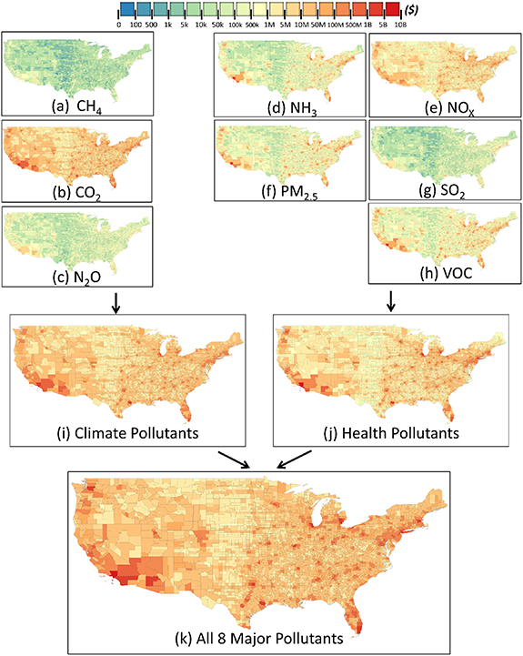
Figure 2. Total social costs attributable to on-road emissions in 2017 for each U.S. county (in $2017 USD). Plotted by pollutant and pollutant category. Pollutant categories include pollutants that contribute to climate change (climate pollutants—CH4, CO2, N2O) and pollutants that directly harm human health through the formation of PM2.5 (health pollutants—NH3, NOx , PM2.5, SO2, VOCs).
Download figure:
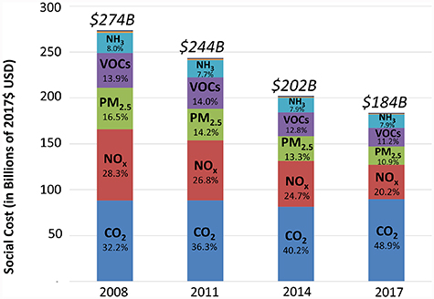
Standard image High-resolution imageCO2 consistently contributed the most social costs each year followed by NOx , PM2.5, VOCs, and NH3 respectively. However, the proportion of total social costs attributable to CO2 greatly increased each year whereas the proportions attributable to all other health pollutants greatly decreased. In fact, CO2's proportion of total social costs in 2017 was approximately 1.5 times what it was in 2008 while PM2.5 and NOx 's proportions in 2017 were approximately two-thirds of what they were in 2008. CH4, N2O, and SO2 contributed negligibly towards the U.S.'s total social costs of transportation (each contributing between 0.1% and 0.6% annually)
Social costs per capita generally vary in different parts of the country but typically have similar magnitude (figure 3). The median social cost per capita attributable to on-road emissions in 2014 was calculated as $578/capita (IQR: $463–$772/capita). Counties with major metropolitan areas did not appear to have relatively different social costs per capita than other parts of the country. Some counties like Orange County (Los Angeles metro area) and Wayne County (Detroit metro area) had social costs per capita of $770 and $783, respectively, but other counties like Miami-Dade County (Miami metro area) and Maricopa County (Phoenix metro area) only had social costs per capita of $395 and $418, respectively. In areas with lower populations but high social costs per capita (such as in the Midwest), it is likely that interstate traffic contributed to proportionally higher social costs per capita.
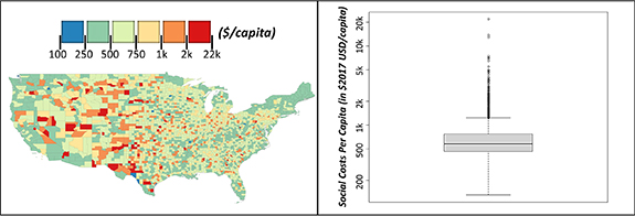
Figure 3. (Left) Total social costs per capita attributable to on-road emissions in 2017 for each U.S. county (in $2017 USD per capita). (Right) The distribution of total social costs per capita that are displayed in the left panel.
Download figure:
Standard image High-resolution image3.3. Emission sources contributing most to social costs
Across all urban, suburban, and rural counties, the average breakdown of vehicle source types contributing to social cost is roughly 65% from individual vehicles, 33% from commercial vehicles, 2% from municipal vehicles, and less than 1% from gas spills. Because municipal and gas spills were small categories, individual and commercial contributions were inversely proportional such that counties with higher than average individual vehicle social cost contributions had lower than average commercial vehicle social cost contributions. The areas with the highest proportion of social costs coming from individual vehicles were counties primarily in New York, New Jersey, Florida, and Oregon with the very highest individual proportions ranging from 83% to 93% of total social costs and the commercial proportions ranging from 5 to 12%. The areas with the lowest proportion of social costs coming from individual vehicles were counties primarily in Texas with the very highest individual proportions ranging from 19% to 35% of total social costs, and the commercial proportions ranging from 62% to 78%.
A table with the summary statistics for total social costs categorized by pollutant, fuel type, urbanicity, and source type is in the supplementary materials for reference (figure S6). The maps in figure 4 have a gradient from urban to rural and another gradient from individual vehicles to commercial, municipal, and then gas spills. Individual vehicles driven in urban counties followed by commercial vehicles driven in urban counties collectively contributed over 80% of the U.S.'s total social costs attributable to on-road emissions.
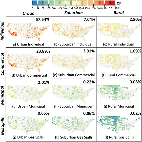
Figure 4. Total social costs attributable to on-road emissions in 2017 for each U.S. county (in $2017 USD). Plotted by vehicle source type (individual, commercial, municipal vehicles, (or gas spills)) and county type (urban, suburban, rural). The percentage in the top right corner of each map indicates the relative contribution of that map to the total social costs attributable to on-road emissions of the eight major pollutants from all county and vehicle source types. Note: all social costs attributable to compressed natural gas (CNG) emissions are excluded from this figure and total to <0.1% of the total social costs.
Download figure:
Standard image High-resolution imageFigure 5 shows the percent of each county's total social costs that are attributable to diesel emissions in 2017. Pollutant-stratified maps that display the percent of total social costs attributable to diesel for each pollutant are in the supplementary materials for reference (figure S7). The percentage of a county's social costs attributable to diesel vehicles ranged from 5% to 78% with most counties having approximately one-third of their social costs from diesel vehicles. For the nation's total social costs, 29% came from diesel vehicle emissions; this proportion has not changed much over the past decade with 32% of total social costs in 2008 coming from diesel.
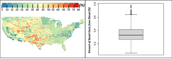
Figure 5. (Left) The percent of total social costs in each U.S. county that are attributable to emissions from diesel vehicles in 2017 (in %). (Right) The distribution of percent of total social attributable to emissions from diesel vehicles that are displayed in the left panel.
Download figure:
Standard image High-resolution imageThe county with the highest social cost, Los Angeles County, contributed slightly greater than 4% of the U.S.'s total social costs from on-road emissions in 2017 (table 1). In addition to Los Angeles County's contribution, the remainder of the top 20 counties collectively contributed an additional 15% of the U.S.'s total social costs. The counties with the highest social cost estimates did not always have the highest social costs per capita. In fact, most of the top counties had a social cost per capita that was within the IQR of $463–$772/capita for all US counties. When we did in-depth analysis on Los Angeles County to understand where the bulk of its social costs were coming from, we found that 75% of total social costs were attributable to health pollutants (versus ∼50% for the full US), and 81% and 16% of total social costs were attributable to individual and commercial vehicles, respectively (versus ∼67% and ∼29% for the full US).
Table 1. Top 20 counties that contributed to the U.S.'s total social costs attributable to on-road emissions in 2017 (in $2017 USD). Metro area, population ranking, and social costs per capita displayed to put high social cost estimates into context.
| Rank | County | Metro area | Population ranking | Social costs per capita | Social cost estimate |
|---|---|---|---|---|---|
| (in $2017 USD) | (in billions of $2017 USD) | ||||
| 1 | Los Angeles | Los Angeles | 1 | 770 | 7.78 |
| 2 | Cook | Chicago | 2 | 694 | 3.61 |
| 3 | Harris | Houston | 3 | 504 | 2.34 |
| 4 | Maricopa | Phoenix | 4 | 419 | 1.81 |
| 5 | Orange | Los Angeles | 6 | 551 | 1.75 |
| 6 | Queens | New York City | 11 | 748 | 1.72 |
| 7 | San Diego | San Diego | 5 | 482 | 1.6 |
| 8 | Dallas | Dallas-Fort Worth | 8 | 580 | 1.52 |
| 9 | Wayne | Detroit | 19 | 783 | 1.38 |
| 10 | Kings | New York City | 9 | 516 | 1.34 |
| 11 | Bergen | New York City | 56 | 1383 | 1.29 |
| 12 | Oakland | Detroit | 32 | 856 | 1.07 |
| 13 | Miami-Dade | Miami | 7 | 395 | 1.07 |
| 14 | St. Louis | St. Louis | 45 | 1073 | 1.07 |
| 15 | King | Seattle | 2 | 484 | 1.07 |
| 16 | Broward | Miami | 17 | 530 | 1.02 |
| 17 | Middlesex | Boston | 22 | 638 | 1.02 |
| 18 | Riverside | Riverside-San Bernardino | 10 | 418 | 1.01 |
| 19 | Tarrant | Dallas-Fort Worth | 15 | 466 | 0.96 |
| 20 | Marion | Indianapolis | 51 | 960 | 0.91 |
Most notable about this table is that the 20 counties listed here can create significant social benefits through policies that reduce VMT simply due to the high emissions currently being produced in each county. If each of these top 20 counties decreased their VMTs such that 10% of CO2 emissions were reduced, they would collectively create a social benefit of nearly $3.4 billion.
3.4. Benefits per ton of CO2 reduced
Health benefits per ton of CO2 reduced varied by a factor of around 7.5, ranging from Los Angeles, CA, New York City, NY, and Chicago, IL with social benefits of between $190 and $369 from a 1 ton reduction of CO2 and its co-pollutants to Aroostook, ME and Washington, ME with social benefits of between $50 and $53 (figure 6).
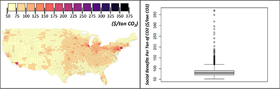
Figure 6. (Left) Total social benefits from reducing 1 ton of CO2 and its co-pollutants from on-road emissions in 2017 for each U.S. county (in $2017 USD ton−1 of CO2). (Right) The distribution of total social benefits in $2017 USD ton−1 of CO2 that are displayed in the left panel.
Download figure:
Standard image High-resolution image4. Discussion
We estimated that the U.S.'s total social costs in 2017 due to on-road emissions were $184 billion ($93 billion for health pollutants; $91 billion for climate pollutants) in $2017 USD (figure 2). These social costs were spread heterogeneously across the 3108 counties in the continental U.S. with the highest social costs from CO2 and NOx emitted from individually owned vehicles in urban counties (figures 2, 4, 7). Emissions have been decreasing overall for most pollutants since 2008 despite overall increases in the number of annual VMT (figure 1, S3); however, increases in population as well as the expansion of new vehicle-reliant industries, such as vehicles supporting oil and gas activity, means that social costs are not guaranteed to continue decreasing, despite past decreases in emissions. Through emissions regulations, standards, policies, and initiatives that reduce on-road emissions of GHGs, health pollutants are simultaneously reduced and health outcomes are consequently improved. While we are not positioning ourselves to make any specific policy recommendations, our analysis can inform the social cost aspect of policy-making decisions. Of course, there are more considerations in policy-making than social costs and benefits, thus other factors such as environmental justice, community cultural behaviors, and technology among other factors should also be considered alongside our social cost analysis when informing policy.
Figure 7. Relative percent contributions of each pollutant to the U.S.'s total social costs attributable to on-road emissions between 2008 and 2017 (in $2017 USD). CH4, SO2, and N2O collectively contribute less than 1.0% of each year's social costs.
Download figure:
Standard image High-resolution image
Total social costs varied substantially by geography. The county with the highest social costs was Los Angeles County, CA which contributed ∼4% of the U.S.'s total social costs from on-road emissions in 2017. Consistent with what we might expect, urban counties had higher social costs due to having larger populations and more on-road vehicles; however, some of the top 20 largest counties did not make the top 20 highest social costs list. Urban counties were responsible for most of the U.S.'s social costs from on-road emissions and generally have higher impacts per capita. This contributes to them having the highest social benefits from reducing 1 ton of CO2 and having the greatest potential social benefits by reducing their emissions even just slightly.
Current literature in the field of social cost estimation typically only discusses the marginal social costs per ton of specific pollutants and rarely combines social cost estimates across multiple pollutants or extrapolates the marginal social costs to provide total social costs as we do in this study. However, we can use published mortality estimates and multiply by the VSL to check that our social cost estimates for health pollutants are reasonable. Caiazzo et al (2013) reported that 53 000 (min: 24 000; max: 95 000) mortalities were due to PM2.5 exposure from on-road emissions in the U.S. in 2005 (Caiazzo et al 2013). When this estimate is adjusted for the same ACS concentration-response function we used and multiplied by a VSL of $9 million ($2017 USD), Caiazzo et al's findings yield $286 billion (min: $130 billion; max: $513 billion) in social costs from on-road health pollutant emissions in 2005. This is in the same range as our social cost estimate for on-road health pollutant emissions in 2008 which was $184 billion (min: $103 billion; max: $288 billion) despite the differences in years of analysis time periods. Additionally, Anenberg et al (2019) reported $210 billion in health damages from PM2.5 and ozone-related premature mortalities in 2015 that is also similar in magnitude to our findings (Anenberg et al 2019). When considering the health benefits per ton of CO2 reduced, Buonocore et al found similar magnitudes of benefits in the range of $0–$100 ton−1 of CO2 for renewable energy initiatives in each region of the US (our estimates ranged mostly from $50 to $125 ton−1 of CO2 for transportation policies that reduce VMT) (Buonocore et al 2019). Our estimates likely are larger because of geographic differences between the electric grid emissions and vehicle emissions—there are more people concentrated where vehicles emit pollutants and less where power plants emit pollutants, thus there is likely to be more of a benefit per ton of CO2 to reduce vehicle emissions than electric grid emissions.
Our analysis has some limitations and uncertainties. The social cost modeling methods inherently adopt uncertainties from their component parts. Any errors in the emissions inventory would affect our results, along with uncertainties of the RCMs, uncertainties in the appropriate discounting rate for GHG social costs, the concentration-response functions, and economic valuation, that all carry into our modeling. However, the model here does scale linearly—so if PM2.5 emissions were found to be underestimated, a different concentration-response function is preferred, or if the VSL were to be revised upward, the effect of any of these changes would scale roughly linearly. That said, if the policy would result in a substantial change in air pollution levels, there could be substantial changes in the CRF as these are not perfectly linear—impact per ton may increase as air quality improves since the CRF exhibits some saturation, since the slope decreases some as air pollution increases (Vodonos et al 2018).
It is worth noting that these social cost estimates refer to damages felt regionally and globally—but are mapped to the origin of emissions. While much of the benefit of air pollution emissions reductions would be felt by communities near the source, much of the benefit will also occur elsewhere. Thus, the costs and benefits of pollution from one county most definitely are felt across the borderlines of counties, and for climate pollutants, across the world. Model frameworks like the Community Multiscale Air Quality Model with Direct Decoupled Method enabled could explicitly estimate these cross-border impacts (Caiazzo et al 2013).
Future areas of research include improving the RCMs and EPA social costs of carbon to include the social costs that are not currently captured and better define the uncertainties of social cost estimation so that we can improve the accuracy of our methods. Of note, the RCMs only incorporate regional health impacts from PM2.5, so impacts of ozone, ultrafine particle exposure, and direct exposure to NO2 and other sources are not included here. The RCMs also only provided monetized estimates of health impacts of mortality, thus missing impacts of other non-fatal health outcomes related to air pollution. Additionally, since the concentration-response function used here is somewhat conservative, factors combined likely make our estimates here highly conservative.
Despite the uncertainties and limitations mentioned above, this paper still provides a robust framework for estimating the climate and health costs of transportation emissions and estimates the benefits of reducing emissions. Our study adds to the growing body of literature that considers both health and climate pollutants from on-road emissions and changes in transportation-related health impacts due to air pollution emissions in the last decade. Recent research generally focuses on either air pollution and health, or climate and only in the capacity of evaluating marginal social costs or mapping emissions—not in calculating the total social costs (Fann et al 2009, Gately et al 2015). This is also the first intercomparison of the three commonly available RCMs applied to the transportation sector, the first nationwide, county-resolution assessment of climate and health impacts of transportation in the U.S., and the first historical reconstruction of the impact of transportation changes in the last decade.
This assessment provides a spatially explicit assessment of health and climate impacts of on-road transportation emissions that can be used to develop interventions by policymakers on the federal, state, and local levels. Our results show which areas and which vehicles classes contribute the highest impact—showing which vehicle types and areas could be prioritized from a climate and health standpoint. Additionally, the benefits per ton of CO2 may provide a reasonable screening estimate of cost-effectiveness per ton of CO2 reduced—a component of developing a health and equity-forward transportation intervention.
5. Conclusion
In this paper, we have mapped out the current state of on-road transportation emissions throughout the U.S. and visually reconstructed trends from the past decade as well as corresponding health impacts. We have identified that the highest social costs from on-road emissions come from CO2 and NOx emitted from individual vehicles in urban counties, and we have quantified other sources' relative contributes to social costs. Additionally, we have assessed the health benefits per ton of CO2 reduced for each county in the continental U.S which policymakers can use as a screening tool for determining the benefits of policies aimed at reducing VMT. The results from this study provide a high-level perspective of the state of transportation emissions in the U.S. that include details of where the most pollutants are being emitted, how emissions have changed over time, and at what social costs. Results indicate that measures in metropolitan counties that reduce VMT will have higher social benefits than in less densely populated counties. This information may be relevant to policymakers both to develop climate and public health impact mitigation strategies, to develop strategies for the transportation sector, determine which regions would benefit most from policy that reduces on-road emissions, and decide which interventions may provide the most benefit for a given region.
Acknowledgments
This work is supported by the Center for Climate, Health, and the Global Environment at the Harvard T H Chan School of Public Health. Special thanks to Dr Gary Adamkiewicz for supporting this work as a faculty advisor and to Drs Francine Laden and John Evans for substantive comments throughout the drafting process.
Data availability statement
The data that support the findings of this study are openly available at the following URL/DOI: www.epa.gov/air-emissions-inventories/national-emissions-inventory-nei.