

Abstract
Understanding the variability of spatial extents of precipitation extremes favors an accurate assessment of the severity of disasters caused by extreme precipitation events. Using a restricted neighborhood method, we identify the spatial extents of global precipitation extremes over 1983–2018 and examine their spatiotemporal variability and associated changes. Results show that the mid-latitudes shows the largest spatial extent of precipitation extremes, and the spatial extents in non-tropical regions over the Northern Hemisphere show significant seasonal differences. In non-monsoon regions, the spatial extents of precipitation extremes in autumn and winter are larger than those in spring and summer, and the annual average spatial extents of precipitation extremes all exceed 500 km, which are larger than those in monsoon regions. All the five non-monsoon regions over the Northern Hemisphere and three monsoon regions in the western Pacific show statistically significant increases in the spatial extent of precipitation extremes in most seasons.
Export citation and abstract BibTeX RIS

Original content from this work may be used under the terms of the Creative Commons Attribution 4.0 license. Any further distribution of this work must maintain attribution to the author(s) and the title of the work, journal citation and DOI.
1. Introduction
Extreme precipitation events can trigger the occurrence of natural disasters such as floods (Luo et al 2018), debris flow (Dowling and Santi 2014, Segoni et al 2015) or landslides (Petley 2012, Tichavský et al 2019), and urban inundation (Yang et al 2016) or waterlogging (Quan et al 2010, Shi et al 2010), and thus bring about huge socio-economic (Tebaldi et al 2006, Schmidt et al 2010, Stocker et al 2013) and ecological (Mullan et al 2012, Woodward et al 2016, Paerl et al 2018) impacts. Precipitation extremes with high intensity and widespread geographical extents and associated extensive flooding can cause transportation disruption, infrastructure damage (Kendon and McCarthy 2015), and a great deal of personnel casualty (Rappaport 2014) in multiple states (Ashley and Ashley 2008) or even multiple countries (Jongman et al 2014) simultaneously, causing much more serious cumulative losses than localized extreme precipitation events. Ignoring the spatial scales of precipitation extremes could lead to the underestimation of the disaster severity (Bevacqua et al 2020). Hence, exploring the spatial extent of precipitation extremes is conducive to studying a basin's hydrological response and the risk management of climate-related extremes (Field et al 2012).
Numerous studies have investigated the characteristic elements of extreme precipitation events and their associated physical mechanisms, but most previous analyses focus on the spatio-temporal variability (Zhang et al 2008, Tabari and Talaee 2011) or changes in the frequency (Kunkel 2003, Jung et al 2011), intensity (Pavan et al 2008, Donat et al 2013, 2016, Tandon et al 2018), and duration (Liu 2011) of precipitation extremes based on precipitation observations (Alexander et al 2006, Peterson et al 2008) or climate model simulations (Tebaldi et al 2006, Sun et al 2007). Analyses of temporal characteristics of precipitation extremes were generally conducted on observed (Zhang and Zhou 2019) and projected (Asadieh and Krakauer 2015, Kitoh and Endo 2016, Zhan et al 2020) precipitation data for each station or grid individually, without considering the co-occurrence of precipitation extremes between neighbor stations and grids. As a regionalized variable, precipitation spreads spatially and shows a certain structure and regional behavior (Al-Khashman and Tarawneh 2007). The spatial characteristics of extreme precipitation events have been studied less systematically, although the spatial extent and the movement of storms are highly important to estimate the flood risk. A recent study shows that the length scale of daily extreme precipitation in summer is about half of that in winter in the eastern US, while seasonal variation is smaller in the western US (Touma et al 2018). Among different types of tropical cyclones, major hurricanes that have weakened to tropical storms can lead to a greater flood risk because of the maximum spatial extent of associated extreme precipitation, although they have weaker wind speeds (Touma et al 2019). A study based on TRMM precipitation radar measurements shows that in tropical and subtropical regions, precipitation over land and maritime continent is generally less extensive than over ocean, but may be more intense when related to mesoscale convective systems (MCSs) and afternoon showers (Hamada et al 2014).
Extreme precipitation events could be intensified and occurred more frequently under a warming climate, as the warmer atmosphere could hold more moisture and precipitable water, thus resulting in more severe precipitation events (Santer et al 2007, Min et al 2011, Stocker et al 2013, Roderick et al 2019). Both observation and model simulations of the historical forcings show that daily extreme precipitation increased on a global scale and there were more increases in the uppermost percentile of the account of precipitation (Allen and Ingram 2002), although changes in precipitation extremes show significantly seasonal and regional differences (Aguilar et al 2005). Exploring how warmer and moister climate modulates the spatial characteristics of precipitation extremes has important implications for projecting the future change in precipitation extremes. Observations in Australia suggest that as temperatures rise, moisture is redistributed and tends to be concentrated near the storm center, leading to a smaller spatial extent of the precipitation (Wasko et al 2016). A study in a business-as-usual warming simulation over the US also reach a similar conclusion that the spatial extent of extreme precipitation events could decrease under a warming climate and the intensity of extreme precipitation increases (Chang et al 2016). However, some results indicate that the storm areas may be larger under climate warming (Lenderink et al 2017, Lochbihler et al 2017). Recent research also found that the total summertime MCS precipitation volume in the US increases by the combined impact of the increase in maximum precipitation rates and the spreading areas of precipitation (Prein et al 2017).
However, these studies mainly investigate the spatial characteristics of precipitation extremes in a specific region (Guinard et al 2015, Wasko et al 2016) or for a specific meteorological cause (Prein et al 2017, Touma et al 2019), or explore its response to warmer climates (Lochbihler et al 2017), which may lead to inconsistent conclusions. The spatiotemporal variability and changes in the spatial extent of global precipitation extremes or its historical climatology have not been investigated. Therefore, this study uses a semi-variogram-based method to identify the spatial extent of global precipitation extremes, and examines the spatiotemporal variability of the spatial extent over 1983–2018 in terms of different regions and seasons, providing the highest-resolution global assessment of spatial extent of daily precipitation extremes. Changes in the spatial extent of precipitation extremes are identified by dividing the precipitation dataset into two non-overlapping periods, 1983–2000 and 2001–2018.
2. Data and methods
The global ground-based precipitation measurements, such as radar or gauges are commonly used to observe global rainfall but sparse and hard to obtain, limiting their ability to capture the spatial details of precipitation extremes (Westrick et al 1999, Ashouri et al 2015). The study of precipitation extremes requires higher spatial resolution because extremes might be smoothed and their intensity dampened in a coarser resolution. At least 30 years of historical weather data are required for climatological studies (Burroughs and Burroughs 2003). Precipitation Estimation from Remotely Sensed Information using Artificial Neural Networks–Climate Data Record (PERSIANN-CDR (Ashouri et al 2015)) is a new retrospective satellite‐based precipitation dataset which is mainly focused on producing climate data record. This dataset provides daily and 0.25° × 0.25° precipitation estimates for the latitude band 60° S–60° N, addressing the need of a consistent, long-term, high-resolution dataset for this study. PERSIANN-CDR is widely used in hydrological (Casse and Gosset 2015, Ashouri et al 2016a), drought (Guo et al 2016), and historical precipitation studies (Nguyen et al 2017, Faridzad et al 2018). PERSIANN-CDR shows outstanding performance in representing characteristics of precipitation extremes and associated changes at fine regional scale (Miao et al 2015, Ashouri et al 2016b, Katiraie-Boroujerdy et al 2017). Thus, we use PERSIANN-CDR on the period from 1983 to 2018 and regard landmass of latitudes from 60° N to 60° S as study regions in this study. We focus on the regional and seasonal characteristics of spatial extends of precipitation extremes, so we compute regional median values in the four seasons (December–January–February, DJF; March–April–May, MAM; June–July–August, JJA; and September–October–November, SON).
To calculate the spatial extents of precipitation extremes in different seasons and in different regions, we define a precipitation extreme as the daily precipitation that exceeds the 90th percentile of each month's daily precipitation on rainy days (>1 mm) from 1983 to 2018 at each grid point. The 90th percentile threshold can satisfactorily represent precipitation extremes that may have significant hydrological effects over most regions around the world (Anagnostopoulou and Tolika 2012), and the 90th percentile threshold keeps a balance between enough exceedances of extreme precipitation and a sufficiently high cut-off value to define extremes. Then we set up a binary dataset to denote the occurrence of precipitation extremes. Specifically, for a grid box, if there is a precipitation extreme on a certain day, it is set as 1 on that day. Otherwise, it is set as 0. If the value at this grid box is missing, it is regarded as a missing value. The binary dataset separates all grid boxes of precipitation extremes from the remaining grid boxes (non-extreme precipitation or missing values).
We use the restricted neighborhood method to identify the spatial extent of precipitation extremes. This method is similar to the moving neighborhood method proposed by Touma et al (2018) and is based on the framework of the semi-variogram function. The estimate of spatial extent is based on the binary dataset we generated previously. We choose 500 km as our neighborhood around a grid box to search for concurrent precipitation extremes. The sensitivity analyses (see text S1 in the supplementary materials (available online at stacks.iop.org/ERL/16/054017/mmedia)) and previously findings shows that the radius of 500 km is sufficient to capture the spatial extent of extreme precipitation generated by different weather systems (Barlow 2011, Smith et al 2011, Catto et al 2012, Catto and Pfahl 2013, Pfahl and Sprenger 2016, Khouakhi et al 2017, Roca et al 2020). For a certain grid box, taking (110.875° E, 27.375° N) as an example, if there is a precipitation extreme (binary value = 1) at this grid box on a day, that grid box is regarded as a center. If there are more than 200 grid boxes around the center, and more than 10% of the grid boxes occurred with precipitation extremes within a radius of 500 km around the center, the semi-variogram is then estimated for this grid box.
We select all grid boxes with a radius of 500 km from the center grid box, pairwise match these grid boxes and classify them into two categories. Category 1–1 means the two paired grid boxes that both occurred with precipitation extremes, while Category 1–0 means only one of the two paired grid boxes that occurred with precipitation extremes, and Category 0–0 is not considered in the analyses. Then we calculate the distances of all pairs in Category 1–1 and category 1–0 respectively, and put them into 40 non-overlapping intervals with 25 km as the equidistant interval (1000 km in total). As shown in figure 1(a), taking 2 days (5 August 2010, and 3 June 2015) as examples, the bars represent the number of pairs in Category 1–1 and Category 1–0 in different intervals. The next step is to calculate the experimental semi-variograms γ(h) in each interval:
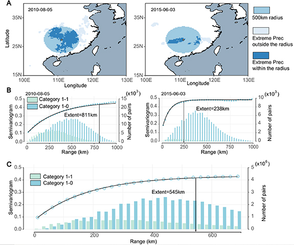
Figure 1. Illustration of the restricted neighborhood method for precipitation extremes spatial extent calculation for a grid box (110.875° E, 27.375° N) in JJA. (a) Take two (05-08-2010; 03-06-2015) of the 198 precipitation extremes in this grid box in JJA as examples to illustrate the restricted neighborhood method. The colors from dark blue to light blue represent the grid boxes occurred with precipitation extremes within the 500 km radius, the grid boxes of 500 km radius from the center (110.875° E, 27.375° N), and the grid boxes occurred with precipitation extremes outside the 500 km radius, respectively. (b) The color bars represent the number of pairs of Categories 1–1 (color in green) and 1–0 (color in blue) in each 25 km interval in these 2 days. The scatters are corresponding experimental semi-variograms and the black lines are the exponential semi-variogram curves fitted. The spatial extents identified are the vertical black lines and ranges showing by the arrows, which are obtained from the fitted semi-variograms. (c) The climatological spatial extent in JJA of this grid box. The color bars represent the cumulative number of all pairs of Categories 1–1 (color in green) and 1–0 (color in blue) from 1983 to 2018 in each interval. The subsequent calculations are as in (b).
Download figure:
Standard image High-resolution imagewhere h is the distance interval, N(h) is the number of pairs (includes Category 1–1 and Category 1–0) in this interval. Z(x), Z(x + h) are the binary values of each pair of grid boxes within the interval, so (Z(x)–Z(x + h))2 is 0 for Category 1–1 and 1 for Category 1–0. γ(h) is the experimental semi-variogram obtained within the interval, and the same calculation was performed for 40 intervals. As shown in the scatter plot in figure 1(a). Finally, the exponential semi-variogram is selected for the experimental semi-variogram fitting, as follows:
where C0 and C is the nugget and partial sill, respectively, which are the initial values that need to be set. a is the range. What we need to focus on is the effective range which means the distance where the semi-variogram reaches 95% of the maximum value and is the spatial extent defined in this study. In an exponential semi-variogram, the effective range is 3a.
For the grid box of 110.875° E and 27.375° N, in JJA from 1983 to 2018, there were a total of 198 precipitation extremes at this grid box. The number of pairs in all intervals neighboring this grid box and corresponding experimental semi-variograms are shown in figure S1. We accumulate the number of pairs of Categories 1–1 and 1–0 from 1983 to 2018 in each season, the experimental semi-variograms are calculated by equation (1) (figure 1(b)), and the exponential semi-variogram is estimated by fitting the data to equation (2), and the effective range is the spatial extent at this grid box in this season (figure 1(c)).
To assess the intra-regional differences in spatial extents within each season and their statistical significance, we use the Wilcoxon rank-sum test (Wilcoxon 1992), in which the spatial extents of precipitation extremes in different regions in each season are independent samples. To similarly access the intra-seasonal differences in spatial extents within each region, we used the Wilcoxon signed-rank test (Wilcoxon 1992), in which the spatial extents of precipitation extremes in different seasons in each region are related samples. For the p values obtained, we calculate the Bonferroni corrected p-values (Sheskin 2000) for pairwise comparisons to increase the strength of the test.
To study changes in spatial extents of precipitation extremes, we divide the entire time series of spatial extent into two time periods, i.e. 1983–2000 and 2001–2018, then separately calculate the spatial extent in each season in these two periods. Taking the first period as a reference, we divide spatial extent values of all grid boxes in the first period into four quartile bins in each region, i.e. the minimum, 25th percentile, the median, the 75th percentile and the maximum spatial extent values. Then the spatial extent percentiles in the second period to identify changes in the spatial extent of each quartile between the two periods. The formula is as follows:
where Epi is the spatial extent value in the second period within quartile bin i of the first period, for example, Ep 1 are the spatial extent values that are greater than the minimum but not greater than the 25th threshold values in the first period. For each region, N is the number of grid boxes in this region, NEpi is the number of selected grid boxes that meet the requirements of this range. qi is the variation of this quartile bin. For all grid boxes in the same region, the Kolmogorov–Smirnov test (Wright 1992) is used to determine whether they are identically distributed between two periods within each season.
3. Results and discussion
3.1. Geographical distribution of precipitation extremes and spatial extent
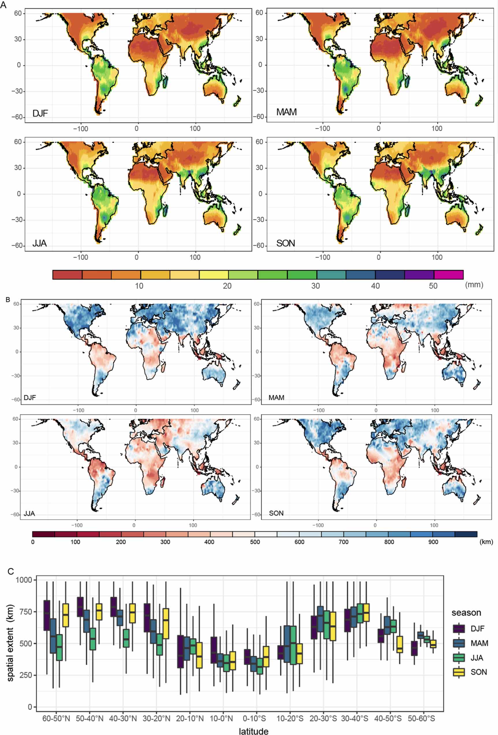
There is generally no substantial seasonal differences in the magnitude (90th percentile values) of precipitation extremes over the global land regions (figure 2(a)), although some regions show significant seasonal differences. In the Northern Hemisphere, larger magnitude of precipitation extremes occurs in boreal summer and autumn than in boreal winter and spring in eastern North America, tropical regions in Africa, Southeast Asia, East Asia and the northern Indian Ocean. The magnitude of precipitation extremes in the southern Himalayas and along the Bay of Bengal in the rainy season is significantly larger than that in the dry season. The magnitude of precipitation extremes in the Southern Hemisphere is consistent in the four seasons. Except in the Indian Ocean, the magnitude of precipitation extremes is larger in the western than the eastern boundary of the oceans. Regions such as the Amazon Basin, Madagascar, southeastern South America and northern Australia show high values of the magnitude of precipitation extremes.

Figure 2. (a) The geographical distribution of seasonal average of the 90th percentile value (mm d−1) of precipitation extremes over 1983–2018 for each season. (b) The geographical distribution of climatological spatial extent of precipitation extremes over 1983–2018 for each season. (c) The box plot for each latitude band of 10° means the climatological spatial extents of all grid boxes in this band for each season, where the 1st, 25th, 50th, 75th and 99th percentile of values are indicated by the bottom vertex of the line, bottom boundary of the box, center line, top boundary of the box and the top vertex of the line, respectively. The median (50th) values is regard as the spatial extent of this latitude band.
Download figure:
Standard image High-resolution imageThe zonal distribution of spatial extent of precipitation extremes is bimodal, in which the mid-latitudes of both the Northern and Southern Hemisphere shows larger spatial extent of precipitation extremes while the mid-high latitudes of the Southern Hemisphere and the tropical latitudes show smaller spatial extent of precipitation extremes (figure 2(c)). The intra-seasonal differences in the spatial extent of precipitation extremes in the mid-latitudes of the Northern Hemisphere are significant, as their differences range 232–265 km. However, the intra-seasonal differences are small in the tropics and throughout the Southern Hemisphere where the differences range only 54–142 km.
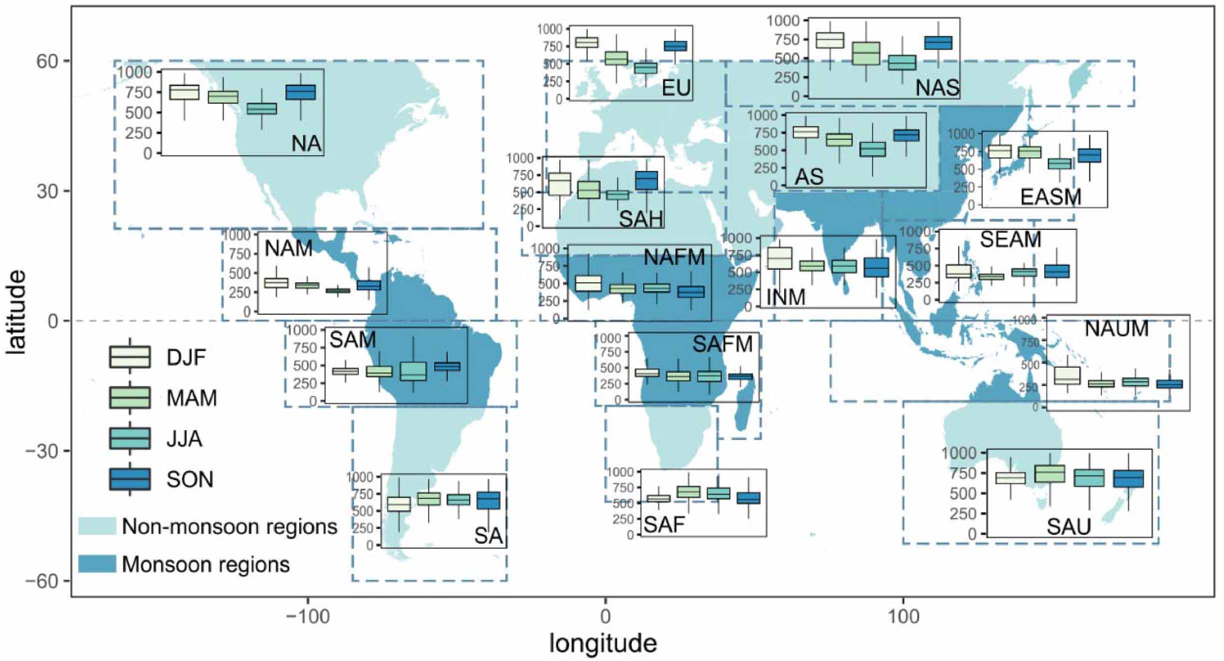
The study regions encompass landmass of latitudes from 60° N to 60° S. We combine the 26 SREX regions proposed by IPCC Special Report on climate extremes (Field et al 2012) with the global monsoon precipitation domain (Wang et al 2012), and divide all land grid boxes into eight monsoon regions and eight non-monsoon regions (figure 3). The location (longitude and latitude coordinates) of the corners of each region are shown in the supplementary material (table S1).
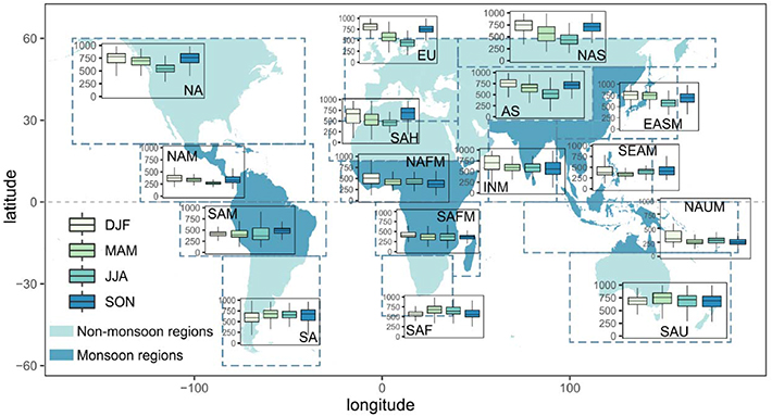
Figure 3. The division of eight monsoon regions (East Asia Monsoon, EASM; Indian Monsoon, INM; Southeast Asia Monsoon, SEAM; North African Monsoon, NAFM; North American Monsoon, NAM; South African Monsoon, SAFM; South American Monsoon, SAM; North Australian Monsoon, NAUM) and eight non-monsoon regions (North America, NA; Asia, AS; North Asia, NAS; Europe, EU; Sahara, SAH; South America, SA; South Africa, SAF; South Australia, SAU). The box plot for each region shows the climatological spatial extents of all grid boxes for each season, where the 1st, 25th, 50th, 75th and 99th percentile of extents are indicated by the bottom vertex of the line, bottom boundary of the box, center line, top boundary of the box and the top vertex of the line, respectively. The median (50th) spatial extent is regard as the spatial extent of this region.
Download figure:
Standard image High-resolution imageIn monsoon regions, the regions of East Asia Monsoon (EASM, 582–752 km) and Indian Monsoon (INM, 553–698 km) show the highest spatial extent of precipitation extremes in all the four seasons (figure 3), with annual average spatial extents of more than 600 km. In other six monsoon regions, the spatial extents are lower than 500 km in all the four seasons. The intra-regional differences between these six regions are all less than 220 km (figure 4(a)). As a tropical region, the precipitation extremes spatial extents of the region of Southeast Asia Monsoon (SEAM) in Asia range from 337 km to 430 km in the four seasons, which are smaller than that of North African Monsoon (NAFM, 370–498 km) and South American Monsoon (SAM, 366–483 km). The spatial extents of precipitation extremes in the region of North American Monsoon (NAM) are lower than that in the region of SAM in all the four seasons, while those in the region of NAFM are higher than in the region of SAFM, especially in the season of SON. The region of North Australian Monsoon (NAUM) shows the lowest spatial extent of precipitation extremes in all monsoon regions, ranging from 255 km to 315 km. Among the four seasons, the maximum intra-regional difference in the season of JJA is the lowest (317 km), while it is over 450 km in DJF and 494 km in MAM, respectively. Generally, the intra-regional differences in the spatial extent of precipitation extremes in the four seasons are statistically significant and show similar ranges in the four seasons (figure 4(a)).
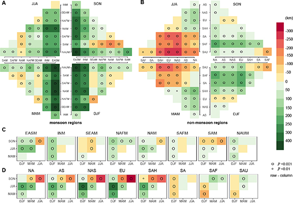
Figure 4. The regional variations and corresponding significance of climatological spatial extents for each season in (a) monsoon regions and (b) non-monsoon regions, and the seasonal variations and corresponding significance of climatological spatial extents for each region in (c) monsoon regions and (d) non-monsoon regions. The colors in tiles represent the differences of median spatial extents. The magnitude of difference is the spatial extent in row region minus that in the column region. The circles inside each tile represent the adjusted p-value of the Wilcoxon rank-sum test in (a) and (b), and of the Wilcoxon signed-rank test in (c) and (d).
Download figure:
Standard image High-resolution imageThe intra-seasonal differences in the spatial extent of precipitation extremes are small in all the eight monsoon regions (figure 4(c)). The difference between the seasons of DJF and JJA in the region of EASM is the largest, up to 172 km, and the maximum intra-seasonal differences in other seven regions are between 46 and 144 km. Most regions in the Northern Hemisphere (except SEAM) show the largest spatial extents of precipitation extremes in boreal winter, but regions of NAUM and SAFM in the Southern Hemisphere show the highest spatial extents in austral summer, and the region of SAM shows the largest spatial extent in austral spring.
Different from the monsoon regions, the annual average spatial extent of precipitation extremes in all non-monsoon regions are all more than 500 km. Sahara (SAH, 470–698 km) is the region of the smallest annual spatial extent (figure 3), while South Australia (SAU, 688–756 km) is the region of the largest spatial extent with an annual average of 709 km, followed by North America (NA, 542–770 km). Regions in the Southern Hemisphere shows the same rank of the spatial extent of precipitation extremes in the regions of SAU, South America (SA), and South Africa (SAF), from the high to low spatial extent, in all the four seasons.
The intra-regional differences in the spatial extent of precipitation extremes are similar between the seasons of DJF and SON, and between the seasons of JJA and MAM, respectively. The spatial extents of precipitation extremes in the Southern Hemisphere are generally larger than those in the Northern Hemisphere regions in the seasons of MAM and JJA, while in the seasons of DJF and SON, the spatial extents in the Northern Hemisphere are generally larger than those in the Southern Hemisphere (figure 4(b)). This phenomenon shows that the spatial extents of precipitation extremes in the non-monsoon regions where are in the local autumn or winter are always larger than those in the non-monsoon regions of the other hemisphere where are in the local spring and summer.
For each region (figure 4(d)), the spatial extents of precipitation extremes in local autumn and winter (SON and DJF for the Northern Hemisphere) are generally larger than those in spring and summer (MAM and JJA for the Northern Hemisphere). The four seasons of DJF, SON, MAM, and JJA, showing from high to low spatial extent in all the five non-monsoon regions in the Northern Hemisphere, show larger intra-seasonal differences in spatial extent. The region of SAH shows a similar spatial extent of precipitation extremes between the seasons of SON and DJF with a difference of only 23 km.
The seasonal differences in spatial extent between local winter and summer in the regions of Europe (EU) and North Asia (NAS) are the largest, reaching 351 km and 312 km, respectively, while those in the other three regions (NA, Asia-AS and NAS) ranges 232–238 km. In three non-monsoon regions in the Southern Hemisphere, the spatial extents in autumn (MAM) are larger than that in other seasons, and the smallest one is in summer or spring (DJF or SON). The intra-seasonal differences in spatial extent in the Southern Hemisphere are small (68–114 km), which is different from the larger difference between boreal summer and winter or autumn in the Northern Hemisphere. In general, both the seasonal and regional differences in the spatial extent of extreme precipitation show asymmetry between the Northern and Southern Hemisphere.
3.2. Changes in spatial extent of precipitation extreme
In monsoon regions, the spatial extents of precipitation extremes in EASM (19–50 km), SEAM (33–69 km) and NAUM (5–65 km) increased in the four seasons, except that in SEAM decreased by 25 km in the season of SON (figure 5), which indicates that the spatial extent of monsoon precipitation extremes over western Pacific increased. On the contrary, the spatial extents of precipitation extremes in INM decreased by 26–72 km in the seasons of MAM, JJA and SON, but that increased by 201 km in DJF. Changes in spatial extents of precipitation extremes over the American (SAM and NAM) and African (SAFM and NAFM) monsoon regions are similar. Specifically, in the regions of SAM and NAM, the spatial extent of precipitation extremes increased in the seasons of DJF and MAM, while in the regions of SAFM and NAFM, the spatial extent of precipitation extremes only increased in JJA and decreased in the other three seasons, although changes are not statistically significant.

Figure 5. Changes in each quartile bin between the first period (1983–2000) and the second period (2001–2018) in each season and in each region. The magnitude of bar in each color shows the quantile in the second period of the spatial extent (the value in the quartile threshold in the first period) minus the corresponding quartile threshold in the first period. The red (blue) numbers show increases (decreases) in the spatial extent of extreme precipitation events.
Download figure:
Standard image High-resolution image
In the non-monsoon regions, the spatial extent of precipitation extremes in the five regions of the Northern Hemisphere increased in the seasons of DJF, MAM, and JJA, even though the seasons of DJF and MAM showed higher increases in the spatial extents of precipitation extremes than those in JJA. The increase in the spatial extent of precipitation extremes in EU (NAS) is up to 190 km (175 km) in MAM, and that in SAH (NAS) is up to 140 km (124 km) in DJF, respectively. In the season of SON, the spatial extents in the four regions of the Northern Hemisphere except NAS decreased by 7–157 km. In the Southern Hemisphere, changes in the spatial extent of precipitation extremes in SA were small (−26–13 km). In the region of SAF, it increased by 123 km in austral winter while decreased by −25 to −57 km in the other three seasons. In the region of SAU, it decreased by 25 km in austral autumn and increased by 35–84 km in the other three seasons.
Changes in the spatial extent of precipitation extremes from the early period to the later period are statistically non-significant (p > 0.01) in only seven regions and in only one season in each region, while changes are statistically significant (p < 0.01) in most regions and most seasons. The changes in the spatial extents of precipitation extremes in most of the regions and in most of the seasons are consistent with changes in the uppermost quartile of the spatial extents of precipitation extremes (q4 in figure 5).
3.3. Implications of changes in spatial extent of precipitation extremes
Regions of the larger magnitude of precipitation extremes are concurrent to regions of a larger spatial extent of precipitation extremes (figures 2(a) and (b)), so there is no positive correlation between the spatial extent and the magnitude of precipitation extremes. This is mainly because the spatial characteristics of precipitation extremes are heavily dependent on specific weather systems, such as tropical cyclones (Knight and Davis 2009, Jiang and Zipser 2010), extratropical cyclones and associated fronts (Catto et al 2012, 2015, Papritz et al 2014), MCSs (Fritsch et al 1986). Large-scale climate modes (DeFlorio et al 2013, Liu et al 2017) such as El Niño–Southern Oscillation, Pacific Decadal Oscillation, and Atlantic Multi-decadal Oscillation also play an important role in forming the environmental conditions triggering above weather systems.
Weather systems associated with extreme precipitation events over various regions show distinct properties in different seasons. Studies found that the mid-latitude extreme precipitation is mainly associated with extratropical cyclones (Hawcroft et al 2012), and the size of extreme precipitation events caused by extratropical cyclone and associated fronts are very large (Hamada et al 2014). Moreover, extratropical cyclone mainly occurs in boreal autumn and winter in the Northern Hemisphere, which is consistent with our result that the spatial extents of precipitation extremes in autumn and winter in non-monsoon regions of the Northern Hemisphere are significantly larger than those in summer. The precipitation features in mid-latitudes are more concentrated in a larger size than those in low latitudes, and they are larger in winter than in summer (Liu and Zipser 2015). Extreme precipitation events in low latitudes is mainly caused by tropical cyclones and convective activities (Liu 2011). Nesbitt et al (2006) defined feature's maximum dimension to assess the spatial extent of tropical and subtropical precipitation, and found that MCSs with a smaller spatial extent contributed more to tropical precipitation, and the tropical spatial features are smaller than the frontal features in subtropics. This is consistent with our result that the spatial extents in monsoon regions (except EASM and INM) are smaller than that in the non-monsoon regions.
There are also some larger MCSs in monsoon season, such as the southeastern United States and Southeast Asia (Liu 2011). In JJA, there are more isolated thunderstorms in the southeastern United States and China, while the Amazon basin and South Africa are dominated by small systems during this local dry season. As a result, precipitation extremes with relatively smaller spatial size contributes more in this season. In DJF, precipitation over the dry region to the north of the intertropical convergence zone in the northeast Pacific is mainly caused by larger precipitation systems. The spatiotemporal patterns of precipitation extremes extents we have found are consistent with these findings.
Further complicating matters, the precipitation mechanism in many regions is related to the topography. For example, precipitation extremes occur frequently in both the Amazon basin and the La Plata basin in southeast South America, but the spatial extent of precipitation extremes in the Amazon basin is much smaller than that in the La Plata Basin. In addition to being related to the convection mechanism in South America, topographic factors such as the Andes also have significant impacts (Romatschke and Houze 2010). Although the mechanisms are beyond the scope of this study, we provide a historical climatology of the spatial extent of precipitation extremes. The corresponding background analyses are suggested for further study. What's more, this study aims to provide a global perspective on the spatial extent of precipitation extremes, but for specific regions, according to the needs of local response to natural disasters, focusing on higher thresholds (95th, 99th, or higher) can capture more intense and localized precipitation and facilitate the study of extreme events that can lead to catastrophic floods and other severe disasters.
4. Conclusions
Using the PERSIANN-CDR precipitation dataset of 1983–2018 (36 years) with a 0.25°  0.25° horizontal resolution and the restricted neighborhood method, we analyze the spatial extent of locally defined daily precipitation extremes which exceed the corresponding 90th percentile value in that grid box. The seasonal and regional features and changes in spatial extents of precipitation extremes are identified. By clustering global landmass grid boxes into eight monsoon regions and eight non-monsoon regions, we assess the intra-regional differences in spatial extent of precipitation extremes within each season and intra-seasonal differences within each region, respectively.
The mid-latitudes of both the Northern and Southern Hemisphere show the largest spatial extent of precipitation extremes. The spatial extents of precipitation extremes in non-monsoon regions are larger than those in monsoon regions, which is mainly manifested in that all the spatial extents in non-monsoon regions exceed 500 km, while those only in monsoon regions of EASM and INM exceed 500 km. The intra-regional differences in spatial extents of precipitation extremes are small in all the four seasons in monsoon regions except EASM. For most of the non-monsoon regions, in the seasons of DJF and SON (JJA and MAM), the spatial extents of precipitation extremes over the Northern Hemisphere are larger (smaller) than those of the Southern Hemisphere.
The spatial extents of precipitation extremes in non-tropical regions over the Northern Hemisphere (NA, EU, NAS, AS, SAH in non-monsoon regions and EASM in monsoon regions) show significant seasonal differences. The maximum seasonal differences in these regions are 180–354 km, and the spatial extents are of the largest value in the season of DJF while that of the smallest ones in the season of JJA. In other four monsoon regions (INM, SEAM, NAM and NAFM) over the Northern Hemisphere and throughout the Southern Hemisphere, the maximum seasonal differences in spatial extent are smaller, ranging from 46 km to 144 km.
To assess changes in spatial extents of precipitation extremes, we divide the time series into two periods (1983–2000 and 2001–2018), then quantify changes in spatial extent in the four quartile bins, respectively. Three monsoon regions (EASM, SEAM and NAUM) which are located in the western Pacific and all the five non-monsoon regions (NA, AS, NAS, EU and SAH) over the Northern Hemisphere show increases (5–190 km) in the spatial extent of precipitation extremes in the seasons of DJF, MAM and JJA except SON. The American monsoon regions (NAM and SAM) in the western Atlantic show increases (6–33 km) in the spatial extent of precipitation extremes in DJF and MAM and decreases (−4 to −73 km) in JJA and SON. In the African monsoon regions (NAFM and SAFM) and SAF in the eastern Atlantic, the spatial extents only increase (3–123 km) in JJA.
Our analyses on the spatial-temporal characteristics of climatological spatial extents of global precipitation extremes have implications for the assessment of disasters caused by precipitation extremes. However, some knowledge gaps remain. To fully explain the inconsistent changes between the magnitude and spatial extent of precipitation extremes, future research should link seasonal precipitation extremes in each region with their meteorological causes, circulation background, and even external forcings.
Acknowledgments
The analysis was financially supported by the National Natural Science Foundation of China (NSFC) (Grant Nos. 51809295, 91547108 and 51779279), Water Science and Technology Innovation Project of Guangdong Province (Grant Nos. 2020–27) and the Guangzhou Science and Technology Plan Project (Grant No. 201904010097). We are very grateful to ComputeCanada for providing the storage and computing resources for this analysis. PERSIANN-CDR data were downloaded from ftp://data.ncdc.noaa.gov/cdr/persiann/files/.
Data availability statement
All data that support the findings of this study are included within the article (and any supplementary files).