


Abstract
Realistically representing the present-day characteristics of extreme precipitation has been a challenge for global climate models, which is due in part to deficiencies in model resolution and physics, but is also due to a lack of consistency in gridded observations. In this study, we use three observation datasets, including gridded rain gauge and satellite data, to assess historical simulations from sixteen Coupled Model Intercomparison Project Phase 6 (CMIP6) models. We separately evaluate summer and winter precipitation over the United States (US) with a comprehensive set of extreme precipitation indices, including an assessment of precipitation frequency, intensity and spatial structure. The observations exhibit significant differences in their estimates of area-average intensity distributions and spatial patterns of the mean and extremes of precipitation over the US. In general, the CMIP6 multi-model mean performs better than most individual models at capturing daily precipitation distributions and extreme precipitation indices, particularly in comparison to gauge-based data. Also, the representation of the extreme precipitation indices by the CMIP6 models is better in the summer than winter. Although the 'standard' horizontal-resolution can vary significantly across CMIP6 models, from ∼0.7° to ∼2.8°, we find that resolution is not a good indicator of model performance. Overall, our results highlight common biases in CMIP6 models and demonstrate that no single model is consistently the most reliable across all indices.
Export citation and abstract BibTeX RIS

Original content from this work may be used under the terms of the Creative Commons Attribution 4.0 license. Any further distribution of this work must maintain attribution to the author(s) and the title of the work, journal citation and DOI.
1. Introduction
Intense precipitation events can lead to flooding, often resulting in infrastructure damage and human casualties, as well as impacts on natural ecosystems, agriculture practice, water resources, and hydroelectric power generation. In the United States (US), these events result in thousands of deaths and billions of dollars in damages annually (Smith and Matthews 2015). Anthropogenic warming and the resulting changes in the climate system can impact the frequency, intensity, spatial extent, duration, and timing of these weather and climate events (IPCC 2013), including increases in the severity of wet and dry precipitation extremes (Easterling et al 2000, Zhai et al 2005, Feng et al 2011). Investigation of such events is important for developing future adaptation strategies (Ren and Chen 2011; Wang and Sun 2012), which are often based on General Circulation Model (GCM) simulation results. Given the growing use of GCMs beyond the scientific community for decision making and impacts applications, it is therefore essential to evaluate their performance. Simulating both the mean climate and extreme events on regional-scales for historical to present-day time periods before assessing projections of future change is crucial (Sillmann et al 2013a). In this study, we focus on precipitation extremes over the US during the recent historical period, with emphasis on daily time-scales, including indices of both wet and dry extremes.
GCMs that have contributed to the Coupled Model Inter-comparison Project Phase 6 (CMIP6, Eyring et al 2016) include higher spatial resolution and additional physical complexity relative to CMIP5 (Taylor et al 2012). However, it is unknown whether these updates improve the representation of the current climate and projections of future changes in precipitation characteristics on regional-scales (Barlow et al 2019; Stegall and Kunkel 2019, Akinsanola and Zhou 2019a; 2019b). Considering the differences among CMIP6 models in representing large-scale dynamics and physical processes, it is expected that model performance may vary over different regions and across both temporal and spatial scales. Globally, there is evidence that GCMs still exhibit long-standing biases in which simulated precipitation occurs more frequently but less intensely than observed (Trenberth 2011), in part due to limitations of convective parameterization and its control on precipitation intensity (e.g. Berg et al 2013), and this behavior is expected to persist. Analysis of CMIP5 models has shown that significant increases in horizontal-resolution (e.g. from ∼2° to ∼0.25°) have a strong impact on the representation of precipitation extremes (e.g. Kopparla et al 2013, Wehner et al 2014); but improvements do not necessarily extend across the entire intensity distribution, since extreme and moderate rates are often controlled separately by resolved synoptic-scale (100–1000 km) and parameterized meso-scale (1–100 km) processes (Kooperman et al 2018). It is also unclear whether moderate increases in resolution, as implemented in some CMIP6 models (e.g. 50–100 km resolution), will better capture meso-scale phenomenon and improve the simulation of the extreme events.
Numerous studies have assessed the performance of CMIP3 and CMIP5 models in simulating precipitation characteristics at global-scales (e.g. Seneviratne et al 2012, Kumar et al 2013, 2014, Pendergrass and Hartmann 2014b, Koutroulis et al 2016, Nguyen et al 2017), but efforts addressing extremes at local and regional scales are less common (e.g. Zhou et al 2014, Sun et al 2015). The goal of this work is to quantitatively evaluate the capability of CMIP6 models in representing the present-day extreme precipitation over the continental US in terms of spatial and temporal variation. We use a standard set of extreme precipitation indices with several readily available observational datasets for comparison. The extreme precipitation indices used herein were defined by the Expert Team on Climate Change Detection and Indices (ETCCDI; Klein Tank et al 2009, Zhang et al 2011). The following sections describe the indices, model simulations, and gridded observations used in our analysis, and an overview and discussion of the results.
2. Data and methodology
2.1. Observations
Previous studies (e.g. Herold et al 2017, Odoulami and Akinsanola 2018) have reported uncertainties and discrepancies between various observation products owing to different data sources and processing algorithms. Hence, we use multiple gridded daily precipitation datasets to evaluate the models' skill in simulating precipitation characteristics for the period of 1997 to 2014. We choose this time period for consistency among all the datasets. The three gridded observations include: National Oceanic and Atmosphere Administration Climate Prediction Center Unified Gauge-Based Analysis resolution (CPC, Chen et al 2008a) at 0.25° × 0.25°; Tropical Rainfall Measuring Mission Multi-satellite Precipitation Analysis (TRMM 3B42 version 7; Huffman et al 2007) at 0.25° × 0.25° resolution, and the Global Precipitation Climatology Project One-Degree Daily product (GPCP 1DD Version 1.2; Huffman and Bolvin 2013). Detailed descriptions of these gridded observations can be found in the review of Sun et al (2018).
2.2. CMIP6 Simulations
The modelled daily precipitation data were obtained from the Earth System Grid data portal and DOE's RGMA archive for the first realization ('r1i1p1f1') from sixteen CMIP6 models (see table 1 for institutions, model names, primary reference, and resolution information of each model). To be consistent with the gridded precipitation datasets, data from 1997 to 2014 from the historical run of the CMIP6 experiment (see Eyring et al 2016 for details of the experiment) were used in this study.
Table 1. Information of the sixteen CMIP6 climate models used in this study.
| S/N | Model | Institute | Resolution (olon × olat) | References |
|---|---|---|---|---|
| 1 | BCC-CSM2-MR | Beijing Climate Center (BCC) and China Meteorological Administration (CMA) | 1.13 × 1.13 | Wu et al (2018) |
| 2 | BCC-ESM1 | Beijing Climate Center (BCC) and China Meteorological Administration (CMA) | 2.81 × 2.81 | Zhang et al (2018) |
| 3 | CanESM5 | Canadan Earth System Model | 2.81 × 2.81 | Swart et al (2019) |
| 4 | CESM2 | National Center for Atmospheric Research | 1.25 × 0.94 | Danabasoglu et al (2019a) |
| 5 | CESM2-WACCM | National Center for Atmospheric Research | 1.25 × 0.94 | Danabasoglu et al (2019b) |
| 6 | CNRM-CM6-1 | Centre National de Recherches Météorologiques (CNRM); Centre Européen de Recherches et de Formation Avancéeen Calcul Scientifique | 1.41 × 1.41 | Voldoire et al (2019) |
| 7 | E3SM | US Department of Energy | 1.25 × 0.94 | Bader et al (2019) |
| 8 | EC-EARTH3 | EC-EARTH consortium | 0.70 × 0.70 | EC-Earth (2019a) |
| 9 | EC-EARTH3-Veg | EC-EARTH consortium | 0.70 × 0.70 | EC-Earth (2019b) |
| 10 | GFDL-CM4 | Geophysical Fluid Dynamics Laboratory (GFDL) | 2.50 × 2.00 | Guo et al (2018) |
| 11 | GFDL-ESM4 | Geophysical Fluid Dynamics Laboratory (GFDL) | 1.25 × 1.00 | Krasting et al (2018) |
| 12 | HadGEM3-GC31-LL | Met Office Hadley Centre | 1.86 × 1.25 | Ridley et al (2019) |
| 13 | IPSL-CM6A-LR | Institute Pierre-Simon Laplace (IPSL) | 2.50 × 1.26 | Boucher et al (2018) |
| 14 | MRI-ESM2-0 | Meteorological Research Institute (MRI) | 1.13 × 1.13 | Yukimoto et al (2019) |
| 15 | SAM0-UNICON | Seoul National University Atmosphere Model Version 0 with a Unified Convection Scheme | 1.25 × 0.94 | Park and Shin (2019) |
| 16 | UKESM1-0-LL | Met Office Hadley Centre | 1.88 × 1.25 | Tang et al (2019) |
2.3. Data processing
For direct comparison of the extreme precipitation metrics, the CMIP6 models and the gridded observation datasets were regridded to a common 2.81° × 2.81° (lat × lon) grid using a remapping procedure which is implemented in the Climate Data Operators (https://code.zmaw.de/projects/cdo) to produce multi-model summary statistics. All the analyses and calculations presented herein are for two seasons: winter (December-January-February, DJF) and summer (June-July-August, JJA). Lastly, the multi-model ensemble mean of all the CMIP6 simulations used in this study, referred to herein as 'EnsMean,' reduces natural variability and systematic biases present in the individual model members (Akinsanola and Zhou 2019c). It is important to note that the distributions and indices are first calculated for the ensemble members individually, and averaged for the EnsMean.
2.4. Rainfall distribution
To provide a broad evaluation of simulated precipitation intensity over the continental US, our initial assessment focuses on area-averaged frequency and amount distributions. The two distributions provide insights not only into the precipitation rates that occur most frequently but also those that contribute the most to seasonal precipitation totals. Previous studies have shown that the distributions of precipitation can be represented in many ways (e.g. gamma (Watterson and Dix 2003), linear (Sun et al 2007, Chou et al 2012), logarithmic (Hennessy et al 1997, Pendergrass and Hartmann 2014a, 2014b)), which are motivated by their application (e.g. mathematical simplicity (Pendergrass and Hartmann 2014a) or interest in the extreme tail of the distribution (Cavanaugh et al 2015)). In this study, a logarithmic bin spacing is applied following Pendergrass and Hartmann (2014a) to capture the full range of rates across orders of magnitude from drizzle to extremes. We adopted the dry day threshold of 0.1 mm day−1, such that the first bin has an approximate width of 0.01 mm day−1, and there are roughly 100 bins that span rates from 0.1 to 1000 mm day−1 (Kooperman et al 2016).
2.5. Extreme precipitation indices
Climate extremes are often studied in one of two ways, either through the use of parametric extreme value theory to assess rare events (Kharin et al 2007, 2013) or using non-parametric indices of climate extremes based explicitly on empirical data (Zhang et al 2011). Here we apply the non-parametric approach using eighteen years of daily data to characterize moderate extreme events (i.e. re-occurrence times within the analysis period, Klein Tank et al 2009) in nine extreme precipitation indices (table 2; for more details see the ETCCDI: http://etccdi.pacificclimate.org/indices_def.shtml) (Karl et al 1999). These indices are derived from daily rainfall and have been widely used in previous studies for detection, attribution, and projection of changes in climate extremes (Dulière et al 2011, Donat et al 2013; Sillmann et al 2013a, Singh et al 2013). The set of indices is related to precipitation occurrence and can characterize flooding and droughts indirectly. These indices are of great interest to a wide range of sectors, especially informative to stakeholders and water resources planners and managers.
Table 2. List of precipitation extreme indices used in this study.
| S/N | Extreme indices | Name | Definition | Units |
|---|---|---|---|---|
| 1 | SDII | Simple daily intensity | Let PRwj be the daily precipitation amount on wet days, PR ⩾ 1 mm in period j. If W represents number of wet days in j, then: SDIIj =  /W /W |
mm/day |
| 2 | CDD | Consecutive dry days | Let PRij be the daily precipitation amount on day i in period j. Count the largest number of consecutive days where PRij < 1 mm | days |
| 3 | CWD | Consecutive wet days | Let PRij be the daily precipitation amount on day i in period j. Count the largest number of consecutive days where PRij > 1 mm | days |
| 4 | PRCPTOT | Total wet-day precipitation | Let PRij be the daily precipitation amount on day i in period j. If I represent the number of days in j, then: PRCPTOTj =  |
mm |
| 5 | R10mm | Heavy precipitation days | Let PRij be the daily precipitation amount on day i in period j. Count the number of days where PRij > 10 mm | days |
| 6 | R20mm | Very heavy precipitation days | Let PRij be the daily precipitation amount on day i in period j. Count the number of days where PRij > 20 mm | days |
| 7 | RX5day | Maximum consecutive 5-day precipitation | Let PRkj be the precipitation amount for the 5-day interval ending k, period j. Then maximum 5 d values for period j are: RX5dayj = max (PRkj) | mm |
| 8 | R95pTOT | Very wet days | Let PRwj be the daily precipitation amount on a wet day w (PR ⩾ 1 mm) in period i and let PRwn95 be the 95th percentile of precipitation on wet days in the 1961–1990 period. If W represents the number of wet days in the period, then: R95pj =  , where PRwj > PRwn95 , where PRwj > PRwn95 |
mm |
| 9 | R99pTOT | Extremely wet days | Let PRwj be the daily precipitation amount on a wet day w (PR ⩾ 1 mm) in period i and let PRwn99 be the 95th percentile of precipitation on wet days in the 1961–1990 period. If W represents the number of wet days in the period, then: R99pj =  , where PRwj > PRwn99 , where PRwj > PRwn99 |
mm |
3. Results
3.1. Seasonal precipitation distributions
In this section, we assess the similarities and differences among the CMIP6 EnsMean and gridded observations (i.e. CPC, TRMM, GPCP) for precipitation frequency and amount distributions over the US in summer and winter seasons (figure 1). At lighter precipitation rates, between 0.1 and 6 mm day−1, the three observations exhibit significant difference; TRMM has a much lower frequency of rain than CPC and GPCP in both seasons (figures 1(a) and (c)). Furthermore, the CPC and GPCP precipitation amount distributions agree broadly in both seasons as they both peak (i.e. the moderate rates that produce the most accumulated precipitation) around 10 mm day−1 and 16 mm day−1 for JJA and DJF, respectively (figures 1(b) and (d)). Precipitation from TRMM observation is more intense than CPC and GPCP in both summer and winter. Specifically, TRMM exhibits a much smaller (higher) amount of precipitation from light (intense) rates, and a moderate precipitation amount peak from heavier rates when compared to the other two observations. The EnsMean rainfall frequency and amount distributions are more consistent in both seasons with CPC and GPCP compared to TRMM, but some biases are evident relative to all three datasets. At lighter precipitation rates, the EnsMean has a much higher frequency of rain than the observations, and nearly twice as frequent as TRMM, for rates as high as 5 mm day−1 and 30 mm day−1 in JJA and DJF, respectively. In summer, the EnsMean amount distribution peak is slightly weak than all observations, but is more consistent with GPCP and CPC during winter. Biases in the total amount of area-average precipitation are also evident in the distributions (e.g. an overall wet bias in winter), but this is discussed with regard to spatial patterns below, since there can be regions of compensating biases.
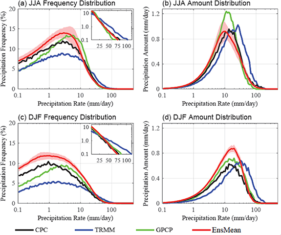
Figure 1. Summer (JJA) and winter (DJF) daily precipitation over the United States for (a & c) precipitation frequency (%) and (b & d) precipitation amount (mm day−1) distributions in CPC, TRMM, GPCP, and CMIP6 models. Small plots in figures 1(a), (c) are frequency distributions shown on a linear axis. Shading is 95% confidence in the CMIP6 models.
Download figure:
Standard image High-resolution imageOverall, CPC and GPCP show better agreement on both the frequency and amount distributions, and the EnsMean is generally more consistent with these two observations than TRMM. The frequency distributions highlight a persistent issue in CMIP6 models that simulate rain too frequently at light rates. However, since light rates do not generate a substantial amount of precipitation, the EnsMean is more consistent with the gridded observations in the amount distribution, which emphasizes heavier rates.
3.2. Mean climatology and precipitation indices
The ability of the CMIP6 EnsMean to represent the spatial characteristics of precipitation over the US is further assessed here. The mean precipitation and four extreme precipitation indices (defined in table 2) are depicted for summer (figure 2) and winter (figure 3) seasons, and for each of the gridded observations and CMIP6 EnsMean over the historical period (1997–2014). We used CPC as the reference dataset to assess model bias, and use the student's t-test to identify regions where CMIP6 EnsMean deviates significantly. CPC was used as the reference data following its remarkable performance over the region as detailed in Sun et al (2018). In fact, cross-validation testing over the continental US suggests that the bias in the CPC observation relative to the mean gauge-observed precipitation is less than 0.5% (Chen et al 2008b). Grid points where differences are statistically significant in the CMIP6 EnsMean dataset are identified with stippling. Although the bias and significance tests are only based on CPC, we include results from all three observations and discuss the difference between them. The three gridded observation datasets are largely consistent in capturing the spatial distribution of daily precipitation in both seasons (figures 2 and 3), although with some noticeable differences. For instance, the amount of precipitation in the TRMM dataset over the southern US is higher than what is observed in CPC and GPCP in JJA season. The noticeable differences between these gridded observations tend to be greatest in regions of high observational uncertainty, especially over the western half of US. Thus, their inclusion is useful for assessing and quantifying the performance of CMIP6 EnsMean against this uncertainty.
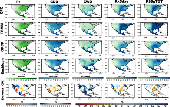
Figure 2. (left)–(right) Mean precipitation and indices CDD, CWD, RX5day, and R95pTOT for summer (JJA) season from (top)–(bottom) CPC, TRMM, GPCP, EnsMean, and bias of EnsMean relative to CPC over the present-day period, 1997–2014. Areas with statistically significant differences are marked with black stippling.
Download figure:
Standard image High-resolution image
Figure 3. Same as figure 2 but for winter (DJF) season.
Download figure:
Standard image High-resolution imageOverall, the CMIP6 EnsMean reproduce the spatial patterns of mean precipitation fairly well (with pattern correlation coefficient (PCC) larger than 0.9 as compared to CPC) and extreme indices in both seasons. As expected, the majority of precipitation is distributed along the southern and eastern (northwestern and eastern) North America in the summer (winter). However, significant biases in the regional magnitudes of these indices are presented in both seasons.
In summer (figure 2), the EnsMean significantly overestimates the seasonal mean precipitation (Pr) over the climatologically dry (wet) northwest US (Mexico) with relative differences reaching 40%–60%. The overestimation in the northwest US is consistent with statistically significant high bias in the length and intensity of precipitation events (CWD and RX5day) and low bias in the length of dry periods (CDD). Further south, in the very dry region of southern California and northern Mexico, there is an underestimation of the seasonal mean precipitation, likely due to a positive (but not significant) CDD bias. Interestingly, the biases over the eastern US also show low CDD and high CWD, but without a mean precipitation bias, due in part to compensating low biases in precipitation intensity. Additionally, the region of more intense rainfall (as represented by Rx5day and R95pTOT) in the Central US (Iowa, Illinois, Minnesota, and Wisconsin), which contributes to high seasonal precipitation amounts (Pr) in the observations (particularly TRMM and CPC), is not reproduced in CMIP6 models, resulting in a dry bias. This is also associated with a noticeable, but not statistically significant, high bias in the number of consecutive dry days in the region.
The observed bias in CWD is evident in majority of the ensemble members (figure S3 (available online at stacks.iop.org/ERL/15/094003/mmedia)), and the regions of significant wet and dry biases in RX5day and R95pTOT are consistent and reproduced fairly well by most of the ensemble members (figures S7 and S8). The spatial correlations of these indices relative to CPC are about 0.91, 0.84, 0.85, and 0.87 for CDD, CWD, RX5day, and R95pTOT respectively.
Furthermore, the spatial biases of SDII, PRCPTOT, R10 mm, R20 mm, and R99pTOT are presented in the supplementary information (figures S1, S4, S5, S6, and S9 respectively ) for the other two gridded observations (GPCP and TRMM), EnsMean, and all the ensemble members. We found a statistically significant dry bias in SDII in the EnsMean over the eastern half of US with high intermodel agreement (figure S1). E3SM, CanESM5 and CESM2 models are the driest among the ensemble members over the region and thus contributes majorly to the signal in EnsMean. While most of the models exhibit dry bias over the eastern half of the US, TRMM exhibits a statistically significant wet bias and thus differ from not only CPC but also GPCP. Considerable biases among the ensemble members, and significant differences in the two observations were also found in other precipitation indices. Wet biases are evident in EnsMean and most of the ensemble members over Mexico, northwest and northeast US in PRCPTOT (figure S4), fairly consistent with the pattern in GPCP but different from TRMM. R10 mm and R20 mm (figures S4 and S5) both exhibit a strong dry bias over the eastern half of the US with high agreement between models. The spatial bias in R99pTOT (figure S9) is quite similar to R95pTOT.
In the winter (figure 3), there is stronger consistency across the precipitation indices assessed here. Simulated precipitation characteristics over the eastern US generally agree with observations, but are grossly exaggerated over the western half of the US. In the west, the CMIP6 EnsMean overestimates total seasonal precipitation (Pr) with associated wet biases in precipitation event length (CWD) and intensity (RX5day and R95pTOT), and a low bias in the length of dry periods (CDD). In fact, all the wet precipitation indices (figures S10, S13–S18) exhibit a strong wet bias that is statistically significant over the western half of US, with high intermodel agreement. This noticeable bias may be related to the representation of orographic processes in the region, which can depend on model resolution, as discussed in Huang and Ullrich (2017). Similar biases in simulating wet extreme precipitation over the topographically complex regions have been reported previously, especially in high-resolution regional climate model (RCM) simulations, and have been primarily attributed to excessively strong winds (Walker and Diffenbaugh 2009, Singh et al 2013). Along the Gulf coast there is also a smaller dry bias that is associated with too little precipitation from longer (Rx5day) and heavier (R95pTOT) events.
Overall, the CMIP6 EnsMean generally captures the patterns of precipitation characteristics, but with notable regional biases. In both seasons, the EnsMean exhibits precipitation events that are too long, with a wet bias in CWD over many parts of the US. Precipitation intensity in the eastern and central US tends to be under-simulated, while the amount and intensity of precipitation is over-stimulated in the west.
3.3. Descriptive statistics and possible impact of resolution
A portrait diagram is a powerful tool in evaluating and summarizing individual models' performance in representing precipitation characteristics with regard to a reference dataset (Sillmann et al 2013a, 2013b). Portrait diagrams for the nine extreme precipitation indices (figure 4) are assessed for the percentage bias, normalized root mean square error, and the pattern correlation coefficient between CPC observations, the other two observations (TRMM and GPCP), and all the CMIP6 models, including their EnsMean. Higher values for most of the extreme precipitation indices are found in both seasons (figures 4(a) and (b)) for TRMM observation, except for CWD and PRCPTOT. The percentage differences exhibited by the GPCP observation relative to CPC are smaller in both seasons. The CMIP6 models exhibit overestimations in the majority of the indices evaluated here, particularly in winter. These include overestimation of CWD, PRCPTOT, R10 mm, and R20 mm (CWD) by the models during winter (summer). The most consistent underestimation is for CDD and SDII in winter and summer, respectively. Generally, there is no single model that performs best for all the nine precipitation indices. Their representation in summer is somewhat better but more variable than in winter. It is worth noting that some moderate and lower resolution GCMs (e.g. SAM0-UNICON, GFDL-ESM4, MRI-ESM2-0, HadGEM3-GC31-LL, GFDL-CM4, BCC-ESM, and CanESM5) exhibit lower percentage biases than many higher resolution models, especially during JJA. Overall, the EnsMean slightly outperforms individual models as a result of the cancellation of spatial errors.
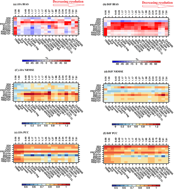
Figure 4. Portrait diagrams showing the percentage bias (a) and (b), normalized root mean square error (c) and (d), and pattern correlation coefficient between CPC observations and all the datasets. The descriptive statistics are for JJA (a), (c) and (e) and DJF (b), (d) and (f).
Download figure:
Standard image High-resolution imageThe normalized root mean square error (NRMSE, figures 4(c) and (d)) is a useful metric to complement the biases discussed above because it is less influenced by spatially compensating errors. NRMSE is uniquely high for R20 mm in both seasons. Since 20 mm day−1 is near the peak in the amount distribution, this may be a moderate rainfall intensity threshold value that models are sensitive to under or over estimating. Overall, the DJF season has lower NRMSE than JJA and the EnsMean also shows remarkably low NRMSE compared to most individual GCMs. Similarly, all the models exhibit pattern correlation coefficients (PCC) that are greater than 0.7 (figures 4(e) and (f)), except for R20 mm which is lower than 0.6 in both seasons. The EnsMean PCC is consistently higher for almost all indices compared to individual models.
Previous studies (e.g. Sillmann et al 2013a; Diaconescu et al 2016) have reported that the performance of models in simulating extreme precipitation indices largely depends upon the choice of the reference dataset. Given this, the portrait diagrams for the nine extreme precipitation indices are further assessed for the percentage bias, normalized root mean square error, and the pattern correlation coefficient using TRMM and GPCP as the reference dataset. Results are presented in figures S20 and S21 respectively. When compared with the TRMM dataset, all the CMIP6 models and the CPC and GPCP gridded datasets exhibit a negative bias in both seasons and most of the indices except CWD and PRCPTOT where a positive bias is observed (figure S20(a) and (b)). These biases are associated with large NRMSE and PCC ∼0.8 in most of the indices (figure S20(c)–(f)). When compared with GPCP (figure S21), the statistics presented in the portrait diagram are very similar to what is observed in figure 4, with all the models exhibiting higher PCC, moderate biases, and lower NRMSE. These results further support our previous findings that the CMIP6 models are more consistent with CPC and GPCP observations than TRMM.
To better understand the possible impacts of moderate differences in resolution, the area-averaged values of the precipitation characteristics over the US in the CMIP6 models were compared with the gridded observations as a function of resolution (figures 5 and S19). The mean values of the precipitation characteristics were plotted against the original resolutions of the observations and models (i.e. resolution before regridding). As stated earlier, we found that some lower and medium resolution models exhibit better performance than some higher resolutions models in representing daily precipitation over the US during summer, although this might not be the case if evaluation is done on their native grid. However, improvement in precipitation indices by horizontal resolution varies with the seasons and the type of extreme precipitation index under consideration. For instance, for CWD all three observations are fairly consistent with each other and tend to be better represented in higher resolution models in both seasons. There is a general trend of lower resolution models having too many consecutive wet days compared to observations. However, very low-resolution models, especially BCC-ESM, do not follow this trend and can be more consistent with observations than some higher resolution models. This is also the case for total seasonal precipitation (Pr), particularly in DJF. There is also a relationship with resolution for other indices, such as Rx5day, but the spread across observations makes it difficult to assess which models perform better.

Figure 5. Area averaged daily precipitation and extreme precipitation indices over the United States vs. model resolutions for JJA (upper panel), and DJF (lower panel) seasons.
Download figure:
Standard image High-resolution image
4. Summary and discussion
Precipitation extremes can have large impacts on society and GCMs can be useful tools for understanding how these extremes may change in the future. However, it is first important to assess how well the newly released CMIP6 models can realistically represent extreme. In this study, we analysed the ability of sixteen CMIP6 models to reproduce present-day precipitation characteristics over the US using a comprehensive set of extreme precipitation indices defined by the ETCCDI and evaluating against several gridded observations. The CMIP6 ensemble mean was found to have a much higher frequency of rain than the observations at lighter precipitation rates, and nearly twice as frequent as TRMM. Other aspects of simulated precipitation distributions for moderate and extreme rates were fairly consistent with CPC and GPCP, but weaker than TRMM. Furthermore, the majority of the ensemble members were found to capture the spatial patterns of mean precipitation and extreme precipitation indices relatively well, but with significant and spatially coherent regional biases. For instance, the EnsMean overestimates the mean precipitation (Pr) in summer over the climatologically dry (wet) northwest US (Mexico), while the intense rainfall center over the Central US could not be reproduced. Also, CMIP6 models generally exhibits too many wet precipitation days (CWD, Pr ⩾ 1 mm day−1). During winter, the largest biases were found for mean precipitation over western half of US, which was grossly exaggerated. This overestimation of winter precipitation and enhanced intensity is also associated with wet biases in CWD, RX5day, and R95pTOT over the same region.
Consistent with previous multi-model ensemble studies (e.g. Sillmann et al 2013a, Zhou et al 2014), the EnsMean generally outperforms any individual model across all the indices considered in this study. The relative performance of an individual model may depend on the choice of the reference dataset. There are significant differences among the available gridded precipitation datasets. However, we found that the CMIP6 models are closer to CPC and GPCP than to TRMM observations over US in terms of spatial representation of precipitation characteristics, NRMSE, percentage bias, and pattern correlation coefficient values. Further analysis showed that the biases in the CMIP6 models may not be alleviated simply by increasing the spatial resolution. In fact, some moderate and lower resolution GCMs exhibit better performance than higher resolution models. Also, when comparing the results of this study to previous assessment of extreme precipitations in CMIP5 (e.g. Sillmann et al 2013a), we found that the spatial biases in most of the indices are relatively similar.
Our study provides a first-order assessment of the CMIP6 model performance in terms of the frequency and amount distributions, and ETCCDI indices over the US. Understanding and removing the sources of bias is a critical next step for improving the accuracy of regional climate prediction. Here we have highlighted season, and areas where CMIP6 models perform well and where they do not, which is important context for assessing confidence in projections of future changes.
Acknowledgments
The authors acknowledge support from the DOE Regional and Global Model Analysis (RGMA) Program (DE-SC0019459) and via NSF IA 1844590. This material is based in part upon work supported by the National Center for Atmospheric Research, which is a major facility sponsored by the National Science Foundation (NSF) under Cooperative Agreement No. 1947282 awarded to AGP. Also, partly performed under the auspices of the U.S. Department of Energy by Lawrence Livermore National Laboratory under Contract DE-AC52-07NA227344. GJK acknowledge support from the University of Georgia's Office of Research, Junior Faculty Seed Grant Program and President's Interdisciplinary Seed Grant Program. We acknowledge the WCRP, which, through its Working Group on Coupled Modelling, coordinated and promoted CMIP6. We thank the modeling groups for producing and making available model output, the ESGF for archiving the data and providing access, and the multiple funding agencies that support CMIP6 and ESGF. We thank DOE's RGMA program area, the Data Management program, and NERSC for making this coordinated CMIP6 analysis activity possible. CPC precipitation data was provided by NOAA/OAR/ESRL PSD. TRMM TMPA 3B42 was provided by the NASA GSFC Mesoscale Atmospheric Processes Laboratory. GPCP 1DD was downloaded from the National Oceanic and Atmospheric Administration /National Centre for Environmental Information.
Data availability
The data that support the findings of this study are openly available.