

Abstract
We investigate the influence of external forcings on the frequency of temperature extremes over land at the global and continental scales by comparing HadEX3 observations and simulations from the Coupled Model Intercomparison Programme Phase 6 (CMIP6) project. We consider four metrics including warm days and nights (TX90p and TN90p) and cold days and nights (TX10p and TN10p). The observational dataset during 1951–2018 shows continued increases in the warm days and nights and decreases in the cold days and nights in most land areas in the years after 2010. The area of the so-called 'warming hole' in North America is much reduced in 1951–2018 compared with that in 1951–2010. The comparison between observation and simulations based on an optimal fingerprinting method shows that the anthropogenic forcing, dominated by greenhouse gases, plays the most important role in the changes of the frequency indices. Changes in CMIP6 multi-model mean response to all forcing need to be scaled down to best match the observations, indicating that the multi-model ensemble mean may have overestimated the observed changes. Analyses that involve signals from anthropogenic and natural external forcings confirm that the anthropogenic signal can be detected over global land as a whole and for most continents in all temperature indices. Analyses that include signals from greenhouse gas (GHG), anthropogenic aerosol (AA) and natural external (NAT) forcings show that the GHG signal is detected in all indices over the globe and most continents while the AA signal can be detected mainly in the warm extremes but not the cold extremes over the globe and most continents. The effect of NAT is negligible in most land areas. GHG's warming effect is offset partially by AA's cooling effect. The combined effects from both explain most of the observed changes over the globe and continents.
Export citation and abstract BibTeX RIS

Original content from this work may be used under the terms of the Creative Commons Attribution 4.0 license. Any further distribution of this work must maintain attribution to the author(s) and the title of the work, journal citation and DOI.
1. Introduction
One of the most visible and serious effects of global warming is the changes in temperature-related extremes, including increases in severe heat waves and decreases in cold surges (Hartmann et al 2013). In the past decades, warm extremes have become more frequent and more intense while cold extremes less frequent and less cold (Donat et al 2013a, Dunn et al 2014, 2020). A global-scale increase in the intensity, duration, and in the number of heat waves has resulted in negative economic, social, and environmental impacts (Wartenburger et al 2017, Sun et al 2018). For example, the European 2003 heat wave killed about 20 000–70 000 people and about 55 000 people died due to the 2010 Russian heat wave (e.g. Wallemacq et al 2018). Because of impacts on society and ecosystems, it is important to understand changes of temperature extremes and related causes.
The World Meteorological Organization (WMO) Expert Team on Climate Change Detection and Indices (ETCCDI) defined a set of indices to describe changes in temperature and precipitation extremes (Zhang et al 2011). These indices, computed from observational data of different regions, show increasing number of warm extremes and decreasing number of cold extremes in past decades over global land (Donat et al 2013a, 2013b, 2016, Alexander 2016) and over continents including Asia (Dong et al 2018), Europe (Christidis and Stott 2016), Australia (Alexander and Arblaster 2017) and other continents (Donat et al 2013b, Alexander 2016). These studies also suggest that changes in nighttime indices are larger than those in daytime indices. Dunn et al (2020) showed warming in temperature extremes continued when recent observational records are added.
Past studies have compared the ETCCDI indices computed from observations with those from simulations by the climate models participating in the 3rd and 5th phases of the Coupled Model Intercomparison Project (CMIP3 and CMIP5, e.g. Morak et al 2013, Bindoff et al 2013). The studies show that CMIP3 and CMIP5 models generally reproduced the observed changes in temperature extremes in the second half of the 20th century at the global scale (Sillmann et al 2013, 2014, Flato et al 2013) and regional scale in some regions (e.g. Alexander and Arblaster 2009, 2017, Morak et al 2013, Dong et al 2018). Evidence has shown that anthropogenic forcing has very likely contributed to the observed changes in the frequency of daily temperature extremes since the 1950s (e.g. Bindoff et al 2013). Morak et al (2011, 2013) find detectable anthropogenic influence in the frequency of warm and cold extremes for different seasons over the globe, the Northern and the Southern Hemispheres and in some sub-continental regions. Christidis and Stott (2016) use simulations by HadGEM2-ES to detect changes in a set of 16 temperature indices. They suggest that, over Europe and global land for the period 1961–2010, anthropogenic forcings could be detected in warm days and nights as well as in cold days and nights, but the natural forcing could not be robustly detected. A series of studies have found detectable anthropogenic signals in the frequency of warm and cold extreme at regional scale over Asia, China, and the Tibetan Plateau (Lu et al 2016, Dong et al 2018, Yin et al 2019). Sun et al (2019) consider the effects of global warming and urbanization and found these two factors can be simultaneously detected in the changes of nighttime temperature extremes but not daytime temperature extremes over Eastern China. Alexander and Arblaster (2009) also investigated the role of anthropogenic forcing in observed changes in temperature extremes over Australia.
While much has been learned about past changes in these temperature extremes indices and their causes, it is an optimum time to revisit this subject for several reasons. The Intergovernmental Panel on Climate Change (IPCC) is conducting its 6th assessment and examining recent advances, thus new studies that make use of recent advances in both observational datasets and climate model simulations are needed to provide input for the assessment. Previous studies are mostly based on HadEX2 dataset (Donat et al 2013a) with 2010 being the last year with data. This dataset has been updated (HadEX3), with extension in temporal coverage to 2018 and improvement in spatial coverage in some regions (Dunn et al 2020). The World Climate Research Program's Coupled Model Intercomparison Project phase 6 (CMIP6, available at https://esgf-node.llnl.gov/projects/cmip6, Eyring et al 2016) has produced a large amount of simulations with the recent generation of climate models. In particular, a CMIP6 endorsed project, the Detection and Attribution Model Intercomparison Project (DAMIP, Gillet et al 2016) was specifically designed to address science questions (among others) related to estimating the contribution of external forcings to observed global and regional climate changes. The DAMIP provides simulations forced with individual external forcing, including historical aerosol-only, stratospheric ozone-only, CO2-only, solar-only, and volcanic-only forcings. These allow us to estimate the separate response from different forcings.
This study takes the advantage of the newly available observational and model data, with an aim to re-examine human influence on four percentile-based frequency indices of temperature extremes at the global and continental scales. We compare changes in extreme temperature indices from updated observations to those computed from the CMIP6 model simulations for 1951–2018, and quantify individual forcing's contribution to the observed changes. The paper is organized as follows. Section 2 describes the datasets and methods used. Section 3 estimates the temporal and spatial variations in temperature extremes, and provides detection and attribution results for various spatial domains including global land and five continents. Conclusion and discussion are given in section 4.
2. Data and methods
2.1. Study region and temperature extreme indices
This study focuses on area averages of the indices over land points of the globe (GLB) and six continents, including Asia (ASI), Europe (EUR), North America (NAM), South America (SAM), Australia (AUS) and Africa (AFR) as defined in Jones et al (2013, figure S1). Based on the ETCCDI definition, the frequency of temperature extremes are represented by percentage of days per year when daily maximum and minimum temperatures are greater than their respective 90th percentiles (TX90p and TN90p) or less than their respective 10th percentiles (TX10p and TN10p) in the base period 1961–1990.
2.2. Observational data
The HadEX3 (available at www.metoffice.gov.uk/hadobs/hadex3) is used to investigate observed changes in the frequency of temperature extremes. This dataset is a global gridded land surface dataset of indices for temperature and precipitation extremes, available on 1.25° × 1.875° latitude-longitude grids and covering 1901–2018 (Dunn et al 2020). We select the grid boxes with sufficient data coverage, defined as grid boxes with at least 70% of data availability during 1951–2018 (i.e. at least 47 years of data) and additionally 3 years of data during 2016–2018 at the minimum. The detection and attribution analyses are conducted for the period 1951–2018 for all continents except South America and Africa. As shown in figure S2, the data coverage is generally good. There is a large data gap in the early period over South America, for this reason, we conduct the detection analyses for South America over the period 1961–2018 (figure S3). The data coverage for Africa is poor and only the northern portion of Africa has sufficient temporal coverage during 1951–2010. For this reason, the African continent is excluded in the detection and attribution analyses. But we will show time series and trends over 1951–2010 in the observations and model simulations as this period has better spatial coverage over the continent. For all the areas, we calculate the anomalies of temperature extremes relative to 1961–1990 at each grid box and then estimate area-weighted regional mean. The linear trends are calculated based on least square method.
2.3. Model data
We use outputs of daily temperatures simulated by the CMIP6 models. The extreme temperature indices are computed using the RClimDex/FClimdex software package (Zhang et al 2011). Historical simulations used in this study include those forced with the combined effect of all forcing (ALL), greenhouse gas forcing (GHG), anthropogenic aerosol forcing (AA) and natural forcing (NAT) over 1951–2018 (table 1). Seven models provide all experiments including historical ALL, GHG, AA, and NAT experiments. These simulations are used to estimate model responses during 1951–2014. The ALL simulations generally end in 2014, but simulations have been extended to 2018 with the SSP2-4.5 scenario by five models, including CanESM5, HadGEM3-GC31-LL, IPSL-CM6A-LR, MRI-ESM2-0 and NorESM2-LM. Simulations by these five models are used to conduct the detection analyses for the period 1951–2018. Unless stated otherwise, the results shown in figures 2–6 are based on these five model results while the seven model detection results for the period 1951–2014 are provided in the Supplementary Information (stacks.iop.org/ERL/15/064014/mmedia) for comparison. The preindustrial control (CTL) experiments by 16 models are used to estimate internal climate variability in the detection and attribution analyses. The CTL simulations are divided into 113 chunks of 68 years (the length of 1951–2018). Model indices are first computed at models' native grid and then bilinearly interpolated onto the 1.25° × 1.875° HadEX3 grids. The regridded data are masked for times and regions where observations are absent to mimic the availability of the observed indices during 1951–2018. The anomalies relative to 1961–1990 mean values at each grid box are calculated and then the regional averages are obtained. The response to anthropogenic forcing (ANT) is estimated as the differences between the model responses to ALL and NAT forcings.
Table 1. List of multimodel simulations used in this study. Numbers represent the ALL, SSP2-4.5, GHG, NAT and AA simulation ensemble sizes or the number of 68-year chunks for the CTL simulations. The ECS and TCR data are from Flynn and Mauritsen (2020).
| model Name | ALL | SSP2-4.5 | GHG | NAT | AA | CTL | ECS(oC) | TCR(oC) |
|---|---|---|---|---|---|---|---|---|
| BCC-CSM2-MRa | 3 | 3 | 3 | 3 | 3.07 | 1.6 | ||
| CanESM5 | 10 | 10 | 10 | 10 | 10 | 11 | 5.58 | 2.75 |
| CNRM-CM6-1a | 3 | 3 | 3 | 3 | 7 | 4.81 | 2.23 | |
| CNRM-ESM2-1 | 7 | 4.75 | 1.82 | |||||
| EC-Earth3 | 7 | |||||||
| EC-Earth3-Veg | 7 | 3.93 | 2.76 | |||||
| GFDL-CM4 | 7 | 3.79 | ||||||
| GFDL-ESM4 | 7 | |||||||
| HadGEM3-GC31-LL | 4 | 4 | 4 | 4 | 4 | 7 | 5.46 | 2.47 |
| INM-CM4-8 | 7 | |||||||
| IPSL-CM6A-LRb | 5/6 | 5/- | 5/6 | 5/6 | 5/6 | 17 | 4.5 | 2.39 |
| MIROC-ES2 L | 7 | 2.66 | 1.51 | |||||
| MIROC6 | 7 | 2.6 | 1.58 | |||||
| MPI-ESM1-2-HR | 7 | |||||||
| MRI-ESM2-0 | 3 | 3 | 3 | 3 | 3 | 2 | 3.11 | 1.67 |
| NorESM2-LM | 3 | 3 | 3 | 3 | 3 | 4 | ||
| UKESM1-0-LL | 2 | 5.31 | 2.79 | |||||
| SUM(models) 1951-2018/1951-2014 | 25(5)/32(7) | 25(5)/- | 25(5)/32(7) | 25(5)/32(7) | 25(5)/32(7) | 113 (16) |
aSimulations of these two models driven by ALL, GHG, NAT and AA are used only for analyses during 1951–2014 in Supplement Information (figures S4–S6). bIPSL-CM6A-LR has five members used for historical ALL(historical and SSP2-4.5), GHG, AA, and NAT simulations during 1951–2018, and six members for historical ALL(historical), GHG, AA, and NAT simulations during 1951–2014.
2.4. Detection methods
We use the regularized optimal fingerprinting method (Ribes et al 2013, Ribes and Terray 2013) to regress the observations onto the signals, i.e. the modelled responses to external forcing. The method is a multivariate linear regression model Y= (X− ν) β +  (Allen and Stott 2003, Ribes et al 2013). The regression coefficients or scaling factors β scale the signals to best match the observations. ν is the sampling noise in the multi-model ensemble mean, and is the regression residual representing internal variability of the climate. A residual consistency test is performed to test the consistency between model-simulated internal variability (estimated from the CTL) and the regression residual. A scaling factor whose 5th percentile is above zero means the corresponding signal is detected at the 5% level. If the 90% range for a
  is above zero and also includes unity, the observed changes are assessed to be consistent with the fingerprint of the external forcing (attribution). If the best estimate of the scaling factor is smaller/larger than unity, it means that the models overestimate/underestimate the response compared to the observations. The detection and attribution analyses are conducted on 5-year mean series of regional mean values. The last data point is the average from values over three year period (2016–2018). We use the regional mean series for the continental analyses. For the global analysis, we conduct space-time analysis by using 5-year mean series from 5 continents (Africa is not included due to lack of data) as 5-spacial dimension.
We conduct single-, two- and three-signal analyses. We only consider ALL forcing in the single-signal analysis because ALL contains all known forcings. For the two-signal analyses, the observations are regressed onto two signals including ANT and NAT, here ANT is computed as the difference between ALL and NAT (i.e. ANT = ALL—NAT). For the three-signal analyses, predictors in the regression include GHG, AA and NAT. In the two- and three-signal detections, if the 90% ranges of  for these predictors are above zero, we claim that they are detected and separated.
3. Results
3.1. Observed and modeled trends
Most previous global and continental analyses of extreme temperature indices are based on HadEX2, and the last year with data in that dataset is 2010. To provide some comparison with earlier results, figure 1 shows trends in the four temperature extreme indices in HadEX3 for two periods 1951–2010 and 1951–2018. There have been increases in the warm days and nights (TX90p and TN90p) and decreases in the cold days and nights (TX10p and TN10p) since 1951 in most land areas, consistent with warming in global mean temperature. For TX90p and TN90p, prominent increases are found in western Europe, most parts of Asia and central part of South America while the decrease in TX90p is seen in south-eastern North America. For TX10p and TN10p, a largest decrease is seen mainly in eastern Russia, China, Mongolia and the central part of South America. For all the warm and cold extremes, the changes in the nighttime extremes (TN90p and TN10p) are larger than corresponding daytime extremes, though they have similar spatial patterns. The trend patterns for the two periods are largely similar, but with some notable differences. The area with cooling trend in southern parts of North America and South America becomes smaller in the longer period, especially for daytime extremes. These indicate that the warming observed in 1951–2010 has persisted and expanded after 2010.

Figure 1. Linear trends in temperature extreme indices for 1951–2018 (top panel) and for 1951–2010 (middle panel) based on HadEX3 data. The lower panel shows the difference between them. The trends are computed only for the grid cells with at least 70% of data available during 1951–2018 and at least 3 years of data during 2016–2018. Blank areas over the land mark regions of insufficient data.
Download figure:
Standard image High-resolution imageFigure 2 shows trends in the observation and the CMIP6 simulations during 1951–2018. The multi-model trends for different forcings are computed as the following: we first compute the medium values of trends of individual model runs for a particular model, 2) the median of these medium values for all models are then taken. The multi-model trends under ALL forcing agree well with the observations in almost all the regions, indicating a good performance of the new generation of climate models in simulating the observed changes in temperature extremes. In the southern part of North America, the ALL results do not reproduce the observed decrease in warm days and the observed increase in cold days. As the cooling area has reduced with additional recent data, that cooling may be more a reflection of natural multi-decadal variability, which is consistent with the study by Kumar et al (2013). The GHG trend patterns are similar to those of ALL, but with larger magnitude of changes in general, indicating stronger warming in the GHG simulations. The AA results show opposite trend but with smaller magnitudes than those of ALL and GHG, indicating cooling effects from anthropogenic aerosols. As for the NAT, it shows quite small trends in the range of −0.2% to 0.2% per decade in most regions, with slight decreases in the warm days and nights and small increases in the cold days and nights, suggesting that the combined effect of the solar irradiance changes and volcanic activities is cooling with very small magnitude. All these indicate that the warming effect of greenhouse gas forcing dominates on the changes in temperature extremes, offset by the cooling effect of anthropogenic aerosols.

Figure 2. Linear trends in temperature extreme indices in HadEX3 (OBS) and in the multi-model simulations under ALL, GHG, AA, and NAT forcing over 1951–2018. The multi-model trends are represented by the medium value of trends computed for individual model from multi-run simulations under each forcing. The trends are computed only for the grid cells with at least 70% of data available during 1951–2018 and at least 3 years of data during 2016–2018.
Download figure:
Standard image High-resolution image3.2. Temporal evolution of temperature extremes
The regional mean time series of the temperature indices and trends in the observations and simulations by the 5 models during 1951–2018 are shown in figure 3. For warm days and nights, there is a clear upward increase over global land and the continents since the 1970s. The largest increase is observed in South America, while the smallest increase is seen in North America. The large linear trends in South America and Africa are related to a large increase since the 1980s. For the cold days and nights, all the regions show decreases after the 1970s. Large decreases in cold nights are seen in South America and Africa while the smallest changes are seen in North America.
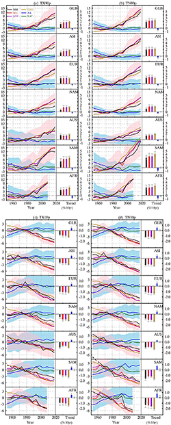
Figure 3. Regional mean 5-yr mean anomalies (relative to the 1961–1990 mean, left) and trends (right) over global land and 6 continents in HadEX3 (OBS) and multi-model ensemble means for (a) TX90p, (b) TN90p, (c) TX10p and (d) TN10p during 1951–2018. The color codes are the following: OBS (black), ALL (red), ANT (estimated from ALL–NAT, purple), GHG (brown), AA (blue) and NAT (green). Regions include global land (GLB), Asia (ASI), Europe (EUR), North America (NAM), Australia (AUS), South America (SAM) and Africa (AFR). The dashed lines for SAM indicate that the HadEX3 data fail to meet the data coverage requirement during 1951–1960. The data for AFR are based on the data coverage during 1951–2010. The pink and blue shadings in the time series plots show the 5%–95% range of the ALL and AA simulations, respectively. Gray error bars on the trend plots show the 5%–95% confidence interval of trend in the observations or 5%–95% spread of trend estimates from available multi-model ensemble runs.
Download figure:
Standard image High-resolution imageFor the model results, the ALL simulations are consistent with the observations in all regions. The GHG results show the largest warming trends while trends from the AA simulations indicate cooling. The absolute magnitude of trend in AA is smaller than that in GHG. There are no clear trends in NAT simulations. Among all the individual forcing simulations, only the GHG simulations are consistent with the observations but both AA and NAT simulations are of opposite sign. This suggests that the observed changes cannot be explained without GHG forcing.
3.3. Single- and two-signal detection results
The best estimates and their 5%–95% confidence intervals of the scaling factors from the single- and two-signal detection analyses are summarized in figure 4. A general impression is that the ALL and ANT signals are robustly detected over global land and almost all the continents. The lower bounds of the 90% confidence intervals of the scaling factors are above zero and most of the residual consistency tests are passed. The confidence intervals for warm extremes are smaller than those for cold extremes, indicating a smaller uncertainty in the estimates associated with warm extremes than cold extremes. For single-signal detection, the best estimates of scaling factors are smaller than unity for most indices in different continents, indicating that models generally have overestimated the observed warming. These values are noticeably smaller than relevant values in Asia from CMIP5 simulations (Dong et al 2018). We note that the CMIP6 models generally have higher climate sensitivity than previous model generations (table 1, Zelinka et al 2020; Flynn and Mauritsen 2020). This suggests that the high sensitivity of the CMIP6 models may also be reflected in their simulated changes in temperature extremes and that the high sensitivity is not realistic. Additionally, changes in aerosol forcing, in particular over Asia in CMIP6 simulations could also play a role. For the two-signal detections, ANT signal can be detected in every region while NAT signal is generally not detected except in NAM. This indicates that the ANT signal plays the dominant role in the changes of warm and cold days and nights. Note that the scaling factor for ANT signal is of similar magnitude to that of ALL, and is smaller than one in almost all cases, indicating once again the models simulate too much warming. These results are consistent with previous results overall, that changes in warm and cold extremes appear to be almost impossible without anthropogenic effect (Morak et al 2011, 2013, Christidis and Stott 2016). We note that NAT signal is generally not detectable in our analysis though it was detected in some of previous studies (Christidis and Stott 2016, Dong et al 2018). The small difference in the results may be due to multiple reasons including differences in datasets, time periods, the details of processing the data, and the fact that the small natural signal is hard to detect because it would need a huge ensemble to provide a robust and clear fingerprint and robust estimate of natural variability (DelSole et al 2019).

Figure 4. Scaling factors and their 5%–95% confidence intervals obtained from the single-signal analyses of ALL forcing and from the two-signal analyses of ANT and NAT forcings for global land (GLB), and 5 continents including Asia (ASI), Europe (EUR), North America (NAM), Australia (AUS) and South America (SAM) for the period 1951–2018. Results for South America are based on data from 1961 to 2018. A downward triangle indicates that the residual consistency test is not passed due to large variability in model simulation and thus the detection results may be conservative.
Download figure:
Standard image High-resolution image3.4. Three-signal detection results
Figure 5 summarizes results from the three-signal analyses. Generally speaking, the GHG signal is detected in almost all the indices over global land and the five continents, with the cold nights (TN10p) over AUS being the exception. The AA signal can be robustly detected over GLB and most continents for warm extremes. The NAT signal is not detected for almost all the regions. For the warm days (TX90p), the GHG and AA can both be detected and separated from each other over GLB and most continents except AUS, but confidence interval for AA in SAM is large. Only GHG signal can be detected over AUS and the NAT signal can be detected only over ASI. For the warm nights (TN90p), the GHG and AA can both be detected over GLB, ASI, EUR and NAM. In other continents, only GHG signals can be detected. These results indicate that when these three signals are taken into account together, the GHG signal is dominant over global land and all continents while AA signal can be robustly detected against noise only over GLB and three of the five studied continents.

Figure 5. Same as figure 4 but for the results from the three-signal analyses.
Download figure:
Standard image High-resolution imageThe detection of the signals in the cold extremes is less often than that in warm extremes. The GHG signal is detected over global land and almost all the continents, except for the cold nights (TN10p) over AUS. However, the residual consistency test failed in this case, indicating the detection is not robust. The best estimate of scaling factor of AA signal is greater than zero for TX10p at 5% significance level over GLB but the residual consistency test did not pass. These do not necessarily indicate that AA signal is weak, rather, they may be a reflection of the difficulties in separating highly co-linear signals in detection and attribution analyses as discussed in previous studies (Jones et al 2013, Schurer et al 2018, DelSole et al 2019). The weak NAT signal cannot be distinguished from internal climate variability in any regions. For the cold nights (TN10p), the models overestimate the observed variability over EUR, NAM and AUS, thus indicating a reduced robustness for the detection results.
Together, the results from three-signal detection and two-signal detection analyses show clearly that GHG is the dominant factor in the observed changes in the frequency of temperature extremes and that the models generally overestimate the response. The AA signal is less detectable, which perhaps is a result of co-linearity with GHG signal. Climate responses to external forcings are easier to detect in warm extremes than in cold extremes. The scaling factors for the globe is very similar to those over Asia and the largest difference between the scaling factors are seen for cold extremes. We also performed the detection analyses based on seven CMIP6 models over the period 1951–2014 (figures S4–S6). The results based on 7 models and the shorter period are quite similar to those based on 5 models with longer period 1951–2018, though it seems that the detectability for some indices in a longer period is slightly higher.
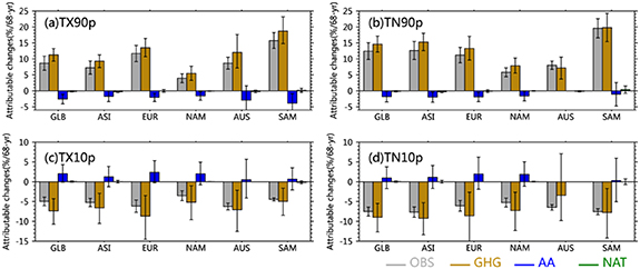
3.5. Attributable changes
The changes in the indices of temperature extremes attributable to GHG, AA and NAT forcings are obtained by multiplying the linear trends in the multi-model mean responses to the corresponding scaling factors estimated in the three-signal analyses (figure 6). Attributable changes are not computed if a scaling factor is negative as that is physically not meaningful. In most cases, the best estimate of the increase in warm extremes attributable to GHG signal is larger than the observed changes, which is offset to a certain extent by the decrease due to AA influence. The NAT signal has also offset slightly the GHG signal over global land. It is estimated that the GHG forcing alone has increased TX90p by 11.2% on global scale (90% confidence interval: 9%–13%), and that this has been offset by 2.5% (1%–4%) by AA's cooling effect and again by 0.2% (0%–0.3%) by NAT forcing. The resulting changes due to the external forcings are very close to the observed change of approximately 8.5% (6%–11%) over 1951–2018.
Figure 6. Trends and their 5%–95% confidence interval (error bars) in the observations (OBS) and that attributable to GHG, AA, and NAT forcings in the extreme temperature indices during 1951–2018. Results for South America are based on data from 1961 to 2018. The attributable trend is estimated by multiplying the linear least squares trends in the relevant signal time series by the corresponding scaling factor. The attributable trend is shown only when the corresponding scaling factor is greater than zero.
Download figure:
Standard image High-resolution image
For the cold extremes, the decrease attributable to GHG forcing is significant but those from AA and NAT forcings are not significant because the relevant scaling factor is not significantly greater than zero or not meaningful to compute as the corresponding scaling factor is negative. For global TX10p, the estimated decrease attributable to GHG signal is about 7% (4%–10%), the observed decrease is 5% (4%–6%), and the estimated increase attributable to AA signal is 2% (0%–4%). However, as the residual consistency test failed in the detection analyses for global TX10p because model simulated variability is large, the corresponding confidence interval of the scaling factor may be conservative. Generally, except the observed change in TN10p over AUS, the GHG induced decrease is slightly more than the observed change in TX10p and TN10p, which has been offset by the increase induced by AA forcing.
4. Conclusion and discussion
We have presented a comprehensive analysis of human influence on the frequency of temperature extremes including TX90p, TN90p, TX10p and TN10p during 1951–2018. Here we compared the observations based on newly available HadEX3 and simulations by CMIP6 models. Previous studies have shown an increase in the warm days and nights and a decrease in cold days and nights in most parts of the world and attribute these changes to human influence (Morak et al 2013, Dunn et al 2020, Alexander 2016). Our study confirms these findings. Additionally, we showed that over the areas where it warmed during 1951–2010 it has warmed at a similar or larger magnitude of warming during 1951–2018 and the size of areas where it cooled in 1951–2010 has reduced in 1951–2018; both indicate continued warming.
The fact that the multi-model mean response to ALL forcing needs to be scaled down to best match the observations indicate that the models may have overestimated the observed warming in the extreme indices. As CMIP6 models have higher sensitivity in general (Flynn and Mauritsen 2020), the overestimation may be related to models' high sensitivity. We find that while effects of ANT and GHG can be detected robustly from the global and continent scales, we have not detected the effect of AA or NAT robustly. In the case of AA, while the effect is strong, we are unable to detect it in many cases. This is largely due to the co-linearity between the GHG and AA signals which degenerates the regression. In the case of NAT, it is mostly due to weak signal.
Acknowledgments
TH and YS are supported by the National Key R&D Program of China (2018YFC1507702, 2018YFA0605604), the National Science Foundation of China (41675074) and the Climate Change Project CCSF201905. SKM and YHK are supported by the Korea Meteorological Administration Research and Development Program under grants KMI2018-01214. We acknowledge the World Climate Research Programme, which, through its Working Group on Coupled Modelling, coordinated and promoted CMIP6. We thank the climate modelling groups for producing and making available their model output, the Earth System Grid Federation (ESGF) for archiving the data and providing access, and the multiple funding agencies who support CMIP6 and ESGF.
Data availability
The data that support the findings of this study are available from the corresponding author upon reasonable request.