

Abstract
Urbanisation is changing the climate of the world we live in. In Great Britain (GB) 5.8% of the total land area is covered by artificial surfaces, increasing from 4.3% in 1975. Aside from associated loss of farmland, biodiversity and a range of ecosystem services, changing to urban form warms the Earth's surface: the urban heat island (UHI) effect. Standard estimates of temperature changes do not account for urbanisation (i.e. use of rural-only stations or removal of urban bias in observations), meaning that anthropogenic modifications to the land surface may be causing the surface-level atmosphere to warm quicker than those estimates suggest. Using observations from a high-density urban monitoring network, we show that locally this warming (instantaneously) may be over 8 °C. Based on the relationships between UHI intensity, urban fraction and wind speed in this network, we create a statistical model and use it to estimate the current daily-mean urban warming across GB to be 0.04 °C [0.02 °C –0.06 °C]. Despite this climate contribution appearing small (94% of GB's land cover for the time-being is still rural), we show that half of GB's population currently live in areas with average daily-mean warming ∼0.4 °C. Under heatwave conditions our high estimates show 40% of GB's population may experience over a 1 °C daily-mean UHI. Furthermore, simply due to urbanisation (1975–2014) we estimate GB is warming at a rate equivalent and in addition to 3.4% [1.9%–5.0%] of the observed surface-level warming calculated from background stations. In the fastest urbanising region, South East GB, we find that these warming rates are up to three times faster. The methodology is straightforward and can be readily extended to other countries or updated as future land cover data becomes available.
Export citation and abstract BibTeX RIS

Original content from this work may be used under the terms of the Creative Commons Attribution 4.0 license. Any further distribution of this work must maintain attribution to the author(s) and the title of the work, journal citation and DOI.
1. Introduction
Since the industrial revolution (∼1760) humanity has transitioned to urban living, with over half the world's population now living in urban areas; up to 80% in more developed regions (United Nations, 2019). Compared to 2000, by 2030 it is estimated that global urban land cover will triple, representing an expansion of 1.2 million km2 (Seto et al 2012). The accompanying reduction in rural land area will not only impact on climate, as explored in this manuscript, but also lead to a significant loss in carbon pools (forests) and biodiversity (Seto et al 2012) and worsen food security (D'Amour et al 2017, Chen et al 2020). Within newly created (and existing) urban regions, a host of major environmental and socio-economic challenges present themselves, such as flooding and poor water quality (Miller and Hutchins 2017), air pollution (Pope et al 2009), and loss of biodiversity (Border et al 2017). Furthermore future projections show urbanisation is unlikely to relent (Chen et al 2020). A further challenge to humanity is the rapidly changing climate around us; impacts are global and the risk from future extremes of temperature and precipitation are only set to worsen (Baker et al 2018). In addition to natural and greenhouse gas drivers of this climate change, replacing vegetated surfaces with urban land cover can lead to a significant warming locally, known as the urban heat island (UHI). The effects of UHIs locally may reach 8 °C (Levermore et al 2018, Chowienczyk et al 2020) and when combined with heatwaves, these can lead to considerable heat-health risks (Heaviside et al 2016, Macintyre et al 2018). However, UHI research is typically confined to the local city of interest, leaving the impacts of anthropogenic land cover modifications to larger-scale climate (in particular from rapid urban expansion) under-evaluated (Pielke et al 2011).
UHIs are product of the built-environments impact on the surface energy balance, largely from reduced albedos; increased heat storage; heat release from buildings, cars and people; reduced sky view factors (proportion of visible sky from the ground); increased surface areas; decreased moisture availability; and back-scattering from air pollution (Arnfield 2003). Aside from urban form, UHI intensities (temperature difference between urban and rural land cover) are influenced by meteorology, with largest intensities usually occurring at night under stable conditions and low wind speeds. Rising warmth from UHIs may also lead to secondary effects, including modifications to atmospheric boundary-layer heights (Barlow 2014), local wind circulations (Hidalgo et al 2010) and increases to downwind precipitation (Han et al 2014). Warmth from UHIs may also be advected significant distances downwind (Bassett et al 2016). UHIs are also not exclusive to large cities, with excess heat detectable even from small urban areas (Hansen et al 2001, Bassett et al 2017).
UHI intensity is known to increase with urbanisation, particularly in rapidly expanding cities (e.g. Ren et al 2007). To date most urbanisation studies focus either on quantifying urban bias within long-term global observation networks or changing UHIs from local growth (i.e. single cities). Urban bias estimates in national temperature networks range from 0.05 to 1.1 °C century−1 (Karl et al 1988, Easterling 1997, Hansen et al 2001, Kalnay and Cai 2003, Li et al 2004, Zhou et al 2004, Ren et al 2008, Sun et al 2016, Shi et al 2019), with the large range arising from different scales of urbanisation in each country. These studies are particularly relevant in certain regions; for example 90% of Chinese meteorological stations are influenced by urbanisation despite urban land only accounting for 1% of the total area (Shi et al 2019). However, these studies do not quantify the overall urbanisation-UHI contribution to climate change, i.e. weighted by regions.
In population terms, our focus country Great Britain (GB; countries of England, Scotland and Wales) is already one of the most urbanised countries in the world with 83% of the population living on 6% of the land (Rae 2017), far higher than the global average urban land cover of 0.5% (Angel et al 2011). Notwithstanding that, the rapid urbanisation rates of many countries worldwide mean their percentage urban land areas are soon likely to surpass that of GB. For the UK (GB plus Northern Ireland), the overall nation-wide nocturnal warming from the UHI effect has recently been estimated at 0.05 °C (Chowienczyk et al 2020), calculated as the difference in interpolated rural observation only and both rural and urban temperature networks. However, this estimate is only for the present-day contribution and does not consider urbanisation trends, which the authors do not think likely to be influential.
In order to reduce heat-health risks and future-proof our cities, accurate wider assessments of urbanisation and its impact on climate are needed; after all, UHI mitigation is possible (Georgescu et al 2014, Wang and Shu 2020). Using a new method in this study, we estimate the overall heat contribution from urban land cover changes to GB climate between 1975 and 2014. We firstly detail the rate of urban expansion during this period using high-resolution land cover maps. A statistical UHI model is then derived using observations from a high-density urban meteorological network, before being scaled (based on the urban land cover maps) to asses GB climate. Our novel approach is straightforward, allowing us to quantify the impact of country-wide urbanisation both spatially and temporally, at scales not usually considered for UHI studies. Moreover, it can be easily be applied to update urbanisation-UHI trend estimates when new land cover data becomes available, or applied to other regions if the data are available.
2. Land cover and meteorological data
Data for assessing GB urbanisation rates in the following section were taken from the Global Human Settlement built (GHS-built) layer covering the periods 1975, 1990, 2000 and 2014 (Corbane et al 2018). Evaluation of GHS-built against ground observations by Pesaresi et al (2016) show improved performance (∼90% accuracy) when compared with similar global land-use products. This is a fine-scale (38 m resolution) global product derived from Landsat images. We aggregated the GHS-built data to 1 km resolution to match the gridded wind speed data described below. Gridded population data were taken from the UK Centre for Ecology and Hydrology, where the 2011 UK Census population data are mapped to 1 km land cover (Reis et al 2017).
The air temperature data for the UHI calculation in section 4 were taken from a high-resolution urban measurement network located in Birmingham, England's second largest city. The Birmingham Urban Climate Laboratory (BUCL) network consisted of 25 Vaisala WXT520 automatic weather stations, supplemented by four UK Met Office weather stations. The network operated across a range of rural and urban land-use types between 2013 and 2014 (see points in figure 1(b)). Metadata for each station are provided in supplementary material table S1 and full details (including quality control procedures) are described by Warren et al (2016). Table S1 also includes the urban fraction (the ratio of urban land cover to the remaining vegetation or water) calculated in a surrounding 500 m radius at each station using the GHS-built data. Although finding representative locations for stations within urban environments represents a challenge, best practices can be adhered to (Muller et al 2013). The BUCL network followed closely to urban observation guidelines proposed by Oke (2007). For example, stations were representative of their local area, not situated on roof tops, and at least 20 m from any point heat sources.

Figure 1. (a) 2014 urban fraction at 1 km resolution derived from the GHS-built data. (b) Subset of (a) located over Birmingham. The blue triangles mark the location of the stations used to calculate the rural reference and black circles mark the remaining locations of the BUCL and Met Office temperature observations. (c) Difference in urban fraction from (b) between 1975 and 2014. Each plot uses the OSGB 1936 coordinate system.
Download figure:
Standard image High-resolution imageTo calculate the meteorological influence on the UHI intensity, daily 10 m wind speed data for GB from 1961 to 2015 were taken from the Climate, Hydrology and Ecology research Support System (CHESS) (Robinson et al 2017). This is a 1 km gridded meteorological and land surface state dataset, downscaled based on topographic information from the 40 km resolution Met Office Rainfall and Evaporation Calculation System data set (MORECS; Hough and Jones 1997). To account for inhomogeneity in wind speed data MORECS standardises each observation to a reference value, that is flat with roughness representing short grass, before interpolation to their grid. Although many wind re-analysis products exist, CHESS was chosen for its combination of high spatial and temporal resolution. The use of a coarser resolution products would not reflect the high variability in wind found at coastal and mountainous regions (De Benedetti and Moore 2020). We checked the data by making a comparison between wind speed taken at Coleshill weather station (located in the BUCL network) and the overlaying CHESS grid cell. A strong (r= 0.93) relationship is found, largely unsurprising considering this is not a truly independent test as the data from the Coleshill station inherently feeds into CHESS. We only note a slight mean wind speed bias of + 0.19 m s−1 in CHESS compared to Coleshill.
3. Urbanisation rates in Great Britain
The near present-day (2014) urban fraction at 1 km resolution across GB is shown in figure 1(a). Overall, 5.8% (or 13 334 km2) of GB's land cover is built-upon. We can see the well-defined cities are largely found in England, South Wales and the Central Belt of Scotland. In England, urban land covers 8.4% of the total land, followed by 3.6% in Wales and 1.4% in Scotland. Within England (but outside of Greater London) the largest urban land area is in the South East, with an urban land fraction of ∼11%.
Table 1 shows the regional changes in urbanisation across GB 1975–2014, which range between 0.1 and 1.4% of the total land area decade−1 (GB mean: 0.37% decade−1). Excluding Greater London, the fastest urbanisation is occurring in the South East of England region (1% decade−1). The rate of urbanisation in GB equates to an area of 86 km2—or nearly the size of Cardiff, Wales—being converted each year. Urban fractions and urbanisation rates in all regions are provided in table 2. Figure 1(c) shows the urbanisation between 1975 and 2014 for the city of Birmingham. Here the fastest urbanisation happened at the city limits; that is, the centre was already heavily urbanised prior to 1975. A similar pattern is found for all other major GB cities. However, our urban land cover data is two dimensional, therefore we do not quantify any vertical growth.
Table 1. Urban fractions for each period by country and English regions, and the decadal mean urbanisation rate (calculated across between 1975 and 2014). All values presented are percentages and urbanisation rate is the percentage of total land area (followed by the 95% confidence intervals). The location of each region is shown in figure 1(a).
| Urban fraction (%) | Urbanisation rate | ||||
|---|---|---|---|---|---|
| 1975 | 1990 | 2000 | 2014 | (% decade−1) | |
| Great Britain | 4.34 | 5.03 | 5.34 | 5.80 | 0.37 ± 0.011 |
| England | 6.53 | 7.57 | 8.07 | 8.36 | 0.47 ± 0.038 |
| Wales | 2.79 | 3.20 | 3.33 | 3.60 | 0.20 ± 0.009 |
| Scotland | 1.05 | 1.23 | 1.29 | 1.44 | 0.10 ± 0.003 |
| North East | 5.57 | 6.06 | 6.29 | 6.76 | 0.30 ± 0.006 |
| North West | 8.57 | 9.81 | 10.30 | 10.74 | 0.55 ± 0.040 |
| Yorkshire and Humber | 6.17 | 6.98 | 7.33 | 7.71 | 0.39 ± 0.021 |
| East Midlands | 4.71 | 5.49 | 5.81 | 6.32 | 0.41 ± 0.014 |
| West Midlands | 7.27 | 8.23 | 8.59 | 9.04 | 0.45 ± 0.026 |
| East of England | 5.21 | 6.28 | 6.96 | 7.92 | 0.69 ± 0.002 |
| Greater London | 62.28 | 64.43 | 65.87 | 67.61 | 1.37 ± 0.016 |
| South East | 7.04 | 8.81 | 9.74 | 10.91 | 0.99 ± 0.027 |
| South West | 3.66 | 4.44 | 4.76 | 5.33 | 0.42 ± 0.012 |
Table 2. Contribution of UHIs to regional and national mean climate in each time period and decadal change. The equivalent percentage of background climate change is calculated using a decadal trend of 0.075 °C.
| Mean UHI contribution (oC) | Mean decadal ΔUHI (oC) | % climate change | ||||
|---|---|---|---|---|---|---|
| 1975 | 1990 | 2000 | 2014 | |||
| Great Britain | 0.030 [0.017 to 0.044] | 0.035 [0.019 to 0.051] | 0.037 [0.021 to 0.055] | 0.040 [0.022 to 0.059] | 0.0026 [0.0014 to 0.0038] | 3.4 [1.9 to 5.0] |
| England | 0.045 [0.025 to 0.067] | 0.052 [0.029 to 0.077] | 0.056 [0.031 to 0.082] | 0.060 [0.034 to 0.089] | 0.0039 [0.0021 to 0.0057] | 5.2 [2.9 to 7.6] |
| Wales | 0.019 [0.011 to 0.028] | 0.022 [0.012 to 0.032] | 0.023 [0.013 to 0.034] | 0.024 [0.013 to 0.036] | 0.0014 [0.0007 to 0.0020] | 1.8 [1.0 to 2.7] |
| Scotland | 0.008 [0.004 to 0.011] | 0.009 [0.005 to 0.013] | 0.009 [0.005 to 0.014] | 0.010 [0.006 to 0.015] | 0.0007 [0.0004 to 0.0010] | 0.9 [0.5 to 1.4] |
| North East | 0.036 [0.019 to 0.053] | 0.039 [0.021 to 0.057] | 0.040 [0.022 to 0.060] | 0.043 [0.023 to 0.064] | 0.0020 [0.0011 to 0.0029] | 2.6 [1.4 to 3.9] |
| North West | 0.060 [0.033 to 0.088] | 0.068 [0.038 to 0.101] | 0.072 [0.040 to 0.105] | 0.075 [0.042 to 0.110] | 0.0039 [0.0022 to 0.0057] | 5.2 [2.9 to 7.7] |
| Yorkshire and The Humber | 0.041 [0.023 to 0.061] | 0.047 [0.025 to 0.069] | 0.049 [0.027 to 0.072] | 0.051 [0.028 to 0.076] | 0.0026 [0.0014 to 0.0038] | 3.5 [1.9 to 5.1] |
| East Midlands | 0.032 [0.018 to 0.048] | 0.038 [0.021 to 0.055] | 0.040 [0.022 to 0.058] | 0.043 [0.024 to 0.063] | 0.0028 [0.0015 to 0.0041] | 3.7 [2.0 to 5.5] |
| West Midlands | 0.049 [0.027 to 0.072] | 0.055 [0.031 to 0.082] | 0.058 [0.032 to 0.085] | 0.061 [0.034 to 0.090] | 0.0031 [0.0017 to 0.0046] | 4.1 [2.3 to 6.1] |
| East of England | 0.035 [0.019 to 0.051] | 0.041 [0.023 to 0.061] | 0.046 [0.025 to 0.068] | 0.052 [0.028 to 0.077] | 0.0045 [0.0024 to 0.0067] | 6.9 [3.3 to 8.9] |
| Greater London | 0.479 [0.278 to 0.697] | 0.495 [0.287 to 0.720] | 0.505 [0.293 to 0.736] | 0.519 [0.301 to 0.755] | 0.0101 [0.0058 to 0.0148] | 13.5 [7.7 to 19.7] |
| South East | 0.052 [0.030 to 0.076] | 0.065 [0.037 to 0.095] | 0.072 [0.041 to 0.105] | 0.081 [0.046 to 0.118] | 0.0073 [0.0042 to 0.0107] | 9.8 [5.6 to 14.3] |
| South West | 0.024 [0.013 to 0.036] | 0.029 [0.016 to 0.043] | 0.031 [0.017 to 0.047] | 0.035 [0.019 to 0.052] | 0.0028 [0.0015 to 0.0042] | 3.7 [2.0 to 5.6] |
4. UHI relationship with urban fraction and wind speed
UHI intensity for Birmingham was calculated by subtracting a rural reference from each station in the BUCL network. The rural reference was taken as the mean of three rural stations (chosen for their low urban fractions): Coleshill, W001, and W003. Prior to calculating the UHI intensity, each station was adjusted to the altitude of the lowest station in the network using the mean environmental lapse rate of 6.5 °C km−1.
Figure 2(a) shows the distribution of hourly UHI intensities at the most urban and warmest station, Paradise Circus. Here, we find a mean intensity of 0.73 °C (s.d. 0.85 °C) during the day and 1.54 °C (s.d. 1.46 °C) at night. Across all time periods the mean is 1.09 °C (s.d. 1.23 °C). Figure 2 shows large distributions of UHI intensity both during the day and at night with the maximum intensity reaching 8.25 °C. UHI intensities of this magnitude are also found in GB cities of London (Chowienczyk et al 2020) and Manchester (Levermore et al 2018). We also note the occurrence of negative UHIs, known as urban cool islands in figure 2. These are a morning feature, arising from the slower urban heating rates caused by increased shading and heat storage capacity (Yang et al 2017).
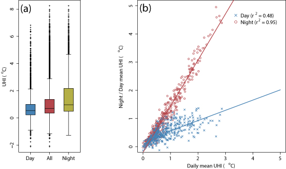
Figure 2. (a) Boxplot showing hourly UHI intensity distribution split into day, night and all cases at the station Paradise Circus. Whiskers are 1.5 x interquartile range. (b) Relationships between daily mean UHI intensity (24 h mean) and 12 h averages of night and day for the recreated urban time series.
Download figure:
Standard image High-resolution imageFrom herein we present analysis for daily time-mean UHI intensity only ( ), i.e. a 24-hour average, to match the temporal resolution of the gridded wind speed we use below. However, as demonstrated in figure 2(a), UHI intensities are modulated by the diurnal cycle, with the largest intensities at night. For reference, figure 2(b) shows the relationships between daily-mean (24-hour) UHI intensity (
 ) and 12-hour averages of either day (
 : 09:00–1800; r2 = 0.48) or night UHI intensity (
 : 18:00–0900; r2 = 0.95). The resulting linear relationships are given by equations (1) and (2):


Figure 3(a) shows a linear relationship between time mean UHI intensity and urban fraction ( ) in the network (r2 = 0.6; note station W011 was considered an outlier and removed from this fit), described by equation (3):

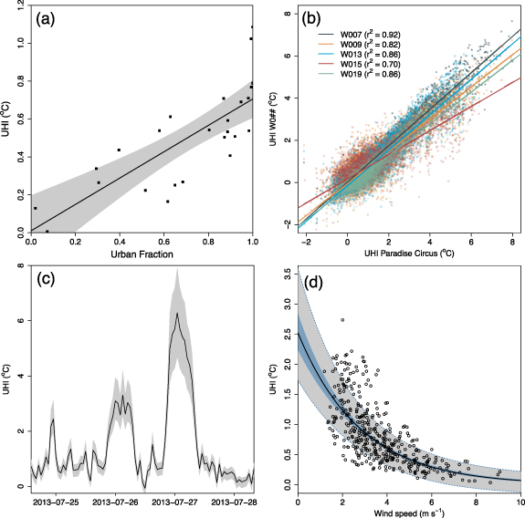
Figure 3. (a) Relationship between urban fraction (calculated in a surrounding 500 m radius from each station) and mean UHI intensity (r2 = 0.6). The grey shading is the 95% confidence intervals of the regression line. (b) Linear relationships between the station Paradise Circus and each of the five next most urban stations (where urban fraction > 0.95). (c) Example period from the recreated UHI intensity time series for urban fractions > 0.95, based on the relationships found in (b). The black line is the mean and grey shading the calculated range (effectively the UHI uncertainty). (d) Daily UHI intensity relationship with wind speed and the mean UHI intensity, using the mean of the recreated time series and wind speed from the CHESS grid cell located over the Coleshill weather station. The solid black line shows the non-linear regression (r2 = 0.6) with the blue shading around it representing the 95% confidence interval. The grey shading is the 95% confidence interval ± the range in UHI uncertainty, that is highlighted in (c).
Download figure:
Standard image High-resolution imageWe note some variability in figure 3(a) between UHI intensity and stations of similar urban fractions. This may be caused by building morphology (e.g. street canyon dimensions) and local heat sources that we are unable to account for in the GHS-built data. The variability may also be caused by stations not always logging simultaneously, meaning that observations may be during periods of different wind speeds and hence UHI intensities. To account for this, figure 3(b) shows the inter-relationship between the six most urban stations, using Paradise Circus (the most consistent records) as a baseline. In figure 3(b) strong linear relationships (r2 = 0.70–0.92) are found between these stations. Therefore, using the resulting linear regression relationships, we created a new UHI time series at each of these stations based on their individual relationship with Paradise Circus. An extract of the resulting time series is shown in figure 3(c), here expressed as a time series of the mean UHI intensity and upper and lower ranges. Using this approach, we find a daily mean (24-hour average) UHI intensity in the observation period for the most urban locations of 0.82 °C, ranging between 0.53 °C and 1.12 °C. Considering all stations have similar urban fractions (>0.95), we consider this range is effectively the uncertainty in our UHI quantification.
The largest UHI intensities are known to occur at low wind speeds (Sundborg 1950, Oke 1973); increased wind speeds and reduced stability effectively disperse UHIs. Using our mean UHI time series we show a non-linear relationship with wind speed (CHESS grid cell located over the Coleshill weather station) in figure 3(d). We map the relationship using a log-linear regression model (see curve in figure 3(d); r2 = 0.59) resulting in equation (4).

Note, outliers with standardised residuals greater than ± 2 sdev were removed prior to the regression. We further represent the uncertainty in the non-linear UHI-wind relationship by adding the range in UHI quantification (see time series in figure 3(c)) on to the 95% confidence interval, see figure 3(d). The remaining urban stations that were not used in the creation of equation (4) were used to evaluate our statistical approach. Across these stations we find a root mean square deviation of 0.17 °C and mean bias error of 0.09 °C between the time-mean observed and predicted UHI intensities. A comparison between our estimate mean UHI intensity and observed UHI intensity at each station is provided in supplementary material figure S1 (stacks.iop.org/ERL/15/114014/mmedia).
5. Scaling the UHI contribution to GB climate
We take the following three steps to generalise the UHI contribution in GB:
- (a)Considering GB experiences large spatial changes in wind speed (a combination of our coasts and hills), we cannot simply apply a single UHI value across all of GB. Therefore, the log-linear relationship from equation (4) is applied daily to each 1 km wind speed grid cell across the 54-year length of the CHESS dataset. We demonstrate in supplementary material figure S2 that the wind speed distribution in the BUCL observation period used to create equation (4) is comparable to the distribution of the 54-year CHESS length.
- (b)For each grid cell we take the mean UHI across 54 years. Although we could have used wind speed data specific to each land cover period, e.g. mean of the 1990 wind speed, different years may have different mean wind speeds, therefore different UHI intensities. To fix this study to impacts of urbanisation only the same wind speed data (54 years) for each land-cover period was therefore used.
- (c)We exploit the clear linear relationship between UHI intensity and urban fraction found in figure 3(a), that is a 1 km grid cell with an urban fraction of 0.5 will have half the UHI intensity of a fully urban cell. This linear relationship is similar in nature to satellite thermal infrared analysis emitted from UK urban areas of different sizes (Abdulrasheed et al 2020). For each period (1975–2014) the UHI results of the first step are weighted by their respective urban fraction.
There are caveats to our approach. Firstly, it assumes that Birmingham's urban land cover is representative of GB, where in reality variations will exist in street canyon dimensions, building materials and morphology, amount of vegetation and moisture availability; however, the thermal properties of UK cities have been shown to be very similar (Abdulrasheed et al 2020). Secondly, it assumes that there are no changes in construction materials or anthropogenic heat fluxes (e.g. increased air conditioning) through the analysis period, and that there have been no large-scale mitigation measures introduced, e.g. cool roofs. Finally, we do not consider any horizontal advection of the UHI. This effect may lead to an underestimation of our UHI climate contribution quantification through: (i) a warming of our rural reference stations, that are located in close proximity to the city, may reduce the calculated urban-rural temperature difference, and (ii) our gridded UHI estimates are not dynamic, i.e. our method would neglect UHI advection from an urban to an adjacent rural grid cell. Therefore, the results of this study provide may only provide a lower estimate of the warming signals and our findings can be improved by further investigations.
Figure 4(a) shows the daily mean results from applying the UHI-wind relationship from equation (4) across GB, prior to weighting by urban fraction. We interpret this as the potential UHI, i.e. the hypothetical daily mean UHI if all land were urban. From this we find an overall potential daily GB mean UHI of 0.64 °C [0.34 °C–0.96 °C]. The values in the square brackets are the UHI uncertainty, detailed in the previous section. Figure 4(a) shows the likely location of highest potential mean UHI intensities to correspond to sheltered valleys and equally lowest UHI intensities to hill tops. Respectively, for the mean case, these account for 5% of values greater than 0.95 °C and 5% less than 0.34 °C. Outside regions of high topographic changes or coasts, we find the highest UHI potential to be inland, particularly southern regions of England. Lower estimates for UHI potential are found in Southwest and Northeast England.
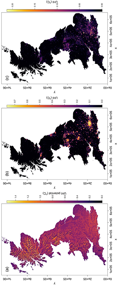
Figure 4. (a) Daily mean UHI potential if GB were completely urban. (b) Present-day (2014) estimated daily mean UHI intensity, i.e. (a) weighted by urban fraction (see figure 1(a)). (c) Change in daily mean UHI intensity 1975–2014. N.b. to improve colour contrast all estimates greater than the 99.9th percentile values are set to this value; these cells being few in number and location confined to sheltered valleys in Scotland.
Download figure:
Standard image High-resolution imageThe daily mean UHI intensity weighted by near present-day (2014) urban fraction is shown in figure 4(b). The largest UHI intensity estimates are found in the cities of London, Manchester and Birmingham with nearly 0.8 °C mean impact on climate. Our estimates are in line with those of Chowienczyk et al (2020), who found a mean UHI intensity of 0.7 °C in Greater London. We found occasional grid cell estimates to exceed UHI intensity values found in cities; however, these are likely a function of low wind speeds in sheltered valleys. Overall the GB daily mean warming (both temporally and spatially) due to the heating from urban land cover is 0.04 °C [0.02 °C–0.06 °C]. This value is similar in magnitude to that of Chowienczyk et al (2020) who estimated a 0.05 °C minimum temperature warming for the UK (GB plus Northern Ireland). Daily mean UHI intensities for each region and period are listed in table 2. Excluding London, South East England experiences the largest daily mean warming at 0.08 °C [0.05 °C–0.12 °C].
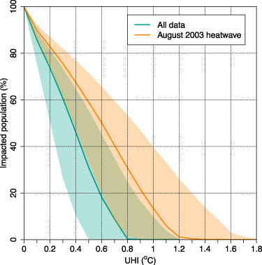
Whilst nationally and regionally our UHI estimates are small, these are spatial means over large areas and GB for the time being is mostly rural (94.2%). Nonetheless, the majority of GB's population live in urban areas. Figure 5 shows the proportion of the GB population impacted by varying degrees of UHI intensity through applying gridded population data (Reis et al 2017). We estimate that over half of GB's 61 million population experiences present-day mean UHIs exceeding 0.37 °C and 15% of the population experience double this. Under the UHI estimates from the upper bound of uncertainty (see bounds figure 3(d)) half of GB's population may experience daily mean UHIs exceeding 0.55 °C and 10% over 1 °C.
Figure 5. The percentage of GB population (total 61 million) impacted the level of UHI intensity. For each the all data (turquoise) and August 2003 heatwave (orange) case the sold line is the mean estimate and grey shading the uncertainty.
Download figure:
Standard image High-resolution image
Furthermore, considering that UHIs combined with heatwaves are known to increase mortality (Heaviside et al 2016) we repeated our calculations for the 3rd—12th August 2003 heatwave, where maximum temperatures in GB reached 38.5 °C (Burt 2004). Under those heatwave conditions, typically periods of stable weather, we estimate that half of GB's population will experience daily mean UHIs greater than 0.6 °C, using the near present-day urban fraction. Using the upper bound of uncertainty (figure 5), during heatwaves of that magnitude, daily mean UHIs exceeding 1 °C could impact nearly 40% of the population. With heatwaves expected to increase in frequency and intensity under climate change (Christidis et al 2020), this stresses the importance of implementing UHI mitigation schemes. Additionally, UHIs are not equally split between day and night (see figure 2), but we can use equations (1) and (2) to approximate their split. A 1 °C daily mean UHI will be 1.4 °C at night and 0.6 °C during the day. These are also daily mean cases, whereas at the hourly scale UHIs may locally exceed 8 °C (see figure 2(a)).
Figure 4(c) shows the change in UHI intensity over 1975–2014. Warming is largely contained around existing settlements, adding approximately 0.1 °C to the local temperature over that time period. Focussing on London, large areas of growth are found to the southwest of the city. Yet, similarly for other major cities, little change is shown in the centre; i.e. it is already saturated with urban land cover. Long-term trend analysis by Jones and Lister (2009) supports this, showing no trend in central London's UHI intensity. However, our UHI estimates for these areas are likely underestimates as we are unable to account for vertical urban growth using the GHS-built (nor anthropogenic heat fluxes) to be accounted for, e.g. replacement of low-rise urban land with skyscrapers. We note the largest change shown in figure 4(c) is growth around the new town of Milton Keynes with almost a 0.2 °C daily mean warming between 1975 and 2014. The significance of the warming for GB overall was tested using the non-parametric Mann–Whitney U test, where a significant difference was found between each case (p < 0.001, n = 230 615).
Within the analysis period, GB urbanisation rates averaged 0.38% per decade, and up to 1% per decade in the South East. Based on our UHI change estimates (ΔUHI) this equates to UHI intensity trends of 0.0026 °C decade−1 [0.0014–0.0038 °C decade−1] for GB as a whole, and three times faster at 0.0073 °C decade−1 [0.0042–0.012 °C decade−1] in the South East. Since 1880 GB has experienced a warming between 0.07 °C decade−1 (Berkley Earth for the UK since 1860; Rohde et al 2013) and 0.08 °C decade−1 (5° x 5° grid cell centred over England; NOAA 2020). Assuming this climate signal contains no urban bias, we infer that simply changing land cover from rural to urban adds an additional 3.4% [1.9%–5.0%] to the GB warming signal (using a central value of GB warming from NOAA and Berkley Earth at 0.075 decade−1). In the South East this additional warming rises to 9.8% [5.6%–14.3%]; values for each region are listed in table 2.
We emphasise our GB-wide urban warming estimates are near-surface level only, i.e. 2 m air temperature, and not representative the whole atmosphere, though warm air is known to rise above cities and increase atmospheric boundary-layer heights (Oke 1982). These decadal estimates are also only valid within the analysis period. For future estimates changes to UHI controlling factors will need to be considered (Mccarthy et al 2010). As most climate statistics avoid use of or bias correct inhomogeneities in their measurements (Menne and Williams 2009, Hansen et al 2010), we argue the overall GB climate is actually warming faster than these trends.
6. Discussion and conclusions
In our study we estimate the warming effect on climate from rapid urbanisation in GB. We explore spatial and temporal scales typically not investigated with urbanisation and UHI studies, which are generally focussed on a single city, or on the urban impact on long-term temperature records. This is achieved by generalising UHI intensity observations from a high-density observation network across GB using a log-linear relationship with wind speed and weighting by urban fraction. We use fixed wind speed data for each land cover period; therefore changes to UHI intensities due to inter-annual climate variability are excluded. Our results show that at the surface level GB as a whole is currently (2014) warmed by 0.04 °C (uncertainty range 0.02–0.06 °C) due to urban land cover, this being similar in magnitude to a recent independent calculation Chowienczyk et al (2020). We extend previous GB-UHI warming estimates by including urbanisation trends, estimating that over 1975–2014 the change in urbanisation alone has caused GB to warm at a rate of 0.0026 °C decade−1 [0.0014–0.0038 °C decade−1]. This warming is more pronounced in some regions of GB, namely the South East, where the warming rate is three times higher. Moreover, if the current rate of urbanisation in the South East continues there will be no green space left in 900 years. While for the whole of GB the urbanisation induced warming is equivalent to 3.4% [1.9%–5.0%] of the observed trends in climate, it is 9.8% [5.6%–14.3%] in the South East. These levels of warming are not insignificant as previously suggested (Chowienczyk et al 2020).
Unlike climate change, warming from urbanisation is theoretically limited, i.e. once all land is urban no further warmer is possible; albeit assuming no changes to urban form, anthropogenic heat fluxes or climate based UHI controls like wind speed (Mccarthy et al 2010). There are also mitigation methods available, like white roofs, to reduce this urban warming (Georgescu et al 2014), and we hope the context of this study will reinforce the need to future-proof cities. Despite the overall spatial mean warming arising from urbanisation being relatively small, UHIs are concentrated in areas where the majority of the population live and work. Indeed we estimate over half of GB's population experience daily mean UHIs greater than 0.37 °C. When combined with existing climate change this will likely lead to exacerbate heat-risks; we already see increased urban mortality during heatwaves (Heaviside et al 2016). Moreover, considering beyond the daily mean, we also demonstrated that UHIs may locally be up to 8 °C. Urbanisation also only forms one component of modification to climate by large-scale land-use changes, with others like deforestation equally as important (Pielke et al 2011).
Overall, we show that urbanisation is contributing to climate change in GB. Considering urbanisation rates in many other countries exceed that found in the UK (e.g. China, India and along the coast of West Africa; Seto et al 2012), the warming we highlight in GB is likely occurring faster elsewhere. Although smaller than the background changes in climate, this warming should not be overlooked, particularly as methods exist to mitigate impacts from urbanisation. However, whilst we make the assumption that Birmingham is broadly representative of urban land cover across GB (itself a limitation), the relationships found here may not be directly applicable to other countries due to differing building materials and morphologies around the world. Nonetheless, providing urban meteorological observations exist, we suggest that the simplicity of our method means estimating urbanisation-induced warming for other countries could be straightforward.
Acknowledgments
This research was made possible through the UK Engineering and Physical Sciences Research Council (EPSRC) Grants EP/N027736/1 (Models in the Cloud: Generative Software Frameworks to Support the Execution of Environmental Models in the Cloud), EP/P002285/1 (The Role of Digital Technology in Understanding, Mitigating and Adapting to Environmental Change) and EP/R01860X/1 (Data Science of the Natural Environment). We would also like to extend our gratitude to the data providers for making this research possible.
Data availability statement
Data that supports the findings of this study are openly available at the following links. High Density Temperature and Meteorological measurements within the Urban Birmingham Conurbation: http://catalogue.ceda.ac.uk/uuid/5391a10e4f644229bc138f8a95ca42f1. Climate, Hydrology and Ecology research Support System (CHESS) 1 km gridded data: https://catalogue.ceh.ac.uk/documents/7de9790e-66a2-44b5-988e-283d764ef52f. Global Human Settlement (GHS) built-up data: http://data.europa.eu/89h/jrc-ghsl-10007. Met Office Integrated Data Archive System (MIDAS) Land and Marine Surface Stations Data (1853-current): http://catalogue.ceda.ac.uk/uuid/220a65615218d5c9cc9e4785a3234bd0. UK gridded population 2011: https://doi.org/10.5285/0995e94d-6d42-40c1-8ed4-5090d82471e1.