

Abstract
Spatiotemporal uncertainty in  emissions in the US hinders prediction of environmental effects of atmospheric
  . We conducted 4D-Var inversions using CrIS remote-sensing observations and GEOS-Chem to estimate monthly
  emissions over the contiguous US at the 0.25°× 0.3125° resolution in 2014, finding they are 33% higher than the prior emissions which likely underestimated most agricultural emissions, especially intense springtime fertilizer and livestock sources over the Central US. However, decreases were found in the Central Valley, southern Minnesota, northern Iowa and southeastern North Carolina during warm months. These updates increased the correlation coefficient between modeled monthly mean
  and surface observations from 0.53 to 0.84, and reduced the normalized mean bias of annual mean simulated
  and wet
  by a factor of 1.3 to 12.7. Our satellite-based inversion approach thus holds promise for improving estimates of
  and reactive nitrogen deposition throughout the world where
  measurements are scarce.
Export citation and abstract BibTeX RIS

Original content from this work may be used under the terms of the Creative Commons Attribution 4.0 license. Any further distribution of this work must maintain attribution to the author(s) and the title of the work, journal citation and DOI.
1. Introduction
As the primary alkaline gas in the atmosphere, ammonia ( ) is an important precursor to fine particulate matter (
 ), and it has effects on soil acidification, ecosystem stability, aerosol acidity, and climate change (Krupa 2003, Myhre et al 2009, Behera et al 2013, Nah et al 2018, Sutton et al 2011).
  emissions are a key factor in
  formation and its reduction has been reported as a cost-effective way to mitigate air pollution (Pinder et al 2007, Wu et al 2016). Additionally, as the increasingly dominant form of reactive nitrogen (Nr) (Du et al 2014, Ellis et al 2013, Li et al 2016),
  plays a significant role in excessive
  and
and  deposition that can harm regional eco-biodiversity through eutrophication and acidification (Erisman et al 2013). To better understand and mitigate the environmental effects of
  , accurate and up-to-date
  emission estimates are required.
Agricultural emissions are the main source of atmospheric  at national scales (Huang et al 2012, EEA 2017, U.S. EPA 2018), although locally non-agricultural sources can dominate (Felix et al 2014, Fenn et al 2018, Berner et al 2020). In the US, agricultural practices (livestock and fertilizer use) account for ∼ 80% of national
  emissions, followed by biomass burning, transportation, industrial activities, residential activities, and other emissions (U.S. EPA 2018). Table 1 shows anthropogenic
  emission inventories for the contiguous US in 2005 to 2014 ranging from 2.4 to 3.40 Tg N a−1 (European CommissionEuropean Commission 2011, Paulot et al 2014, Janssens-Maenhout et al 2015, Crippa et al 2018, Hoesly et al 2018). This large uncertainty in
  emission inventories is due to scarce measurements of locally representative emission factors and out-of-date activity data (Beusen et al 2008, Holt et al 2017).
Table 1.  emission estimates (Tg N a−1) for the contiguous US.
| Literature | Target year | Anthropogenic  emissions emissions |
|---|---|---|
| Bottom-up | ||
| NEI2008 | 2006 | 3.1 |
| Paulot et al (2014) | 2005-2008 | 2.4a |
| EDGAR v4.2 | 2008 | 2.9 |
| EDGAR v4.3.2 | 2010 | 3.40c |
| HTAP v2 | 2010 | 2.95 |
| CEDS_2018 | 2014 | 3.05 |
| Top-down | ||
| Zhang et al (2012) | 2006-2008 | 2.3 |
| Paulot et al (2014) | 2005-2008 | 2.8b |
| Dammers2019 | 2013-2017 | 1.07d (2.9 times HTAP v2) |
| This study | 2014 | 3.91 |
aBottom-up anthropogenic  emissions, with agricultural emissions taken from MASAGE inventory.
bTotal
emissions, with agricultural emissions taken from MASAGE inventory.
bTotal  emission (anthropogenic + biomass burning + natural sources) estimate derived from NADP wet
  deposition measurements.
cIncluding
deposition measurements.
cIncluding  emissions from agricultural soils (AGS), agricultural waste burning (AWB), manure management (MNM), chemical processes (CHE), power industry (ENE), combustion for manufacturing (IND), non-metallic minerals production (NMM), energy for buildings (RCO), oil refineries and transformation industry (REF_TRF), solid waste incineration (SWD_INC), solid waste landfills (SWD_LDf), shipping (TNR_Ship), railways,pipelines, off-road transport (TNR_Other), Road transportation (TRO), waste water handling (WWT) (Crippa et al 2018).
dOnly
emissions from agricultural soils (AGS), agricultural waste burning (AWB), manure management (MNM), chemical processes (CHE), power industry (ENE), combustion for manufacturing (IND), non-metallic minerals production (NMM), energy for buildings (RCO), oil refineries and transformation industry (REF_TRF), solid waste incineration (SWD_INC), solid waste landfills (SWD_LDf), shipping (TNR_Ship), railways,pipelines, off-road transport (TNR_Other), Road transportation (TRO), waste water handling (WWT) (Crippa et al 2018).
dOnly  emissions from 48 large point-sources (mainly industrial and agricultural sources) over North America.
Alternatively, observations of  and its reaction products (i.e.
  ) can provide top-down constraints on
  sources. In-situ wet deposition measurements were first used to constrain the seasonal cycle and magnitude of US
  emissions by Gilliland et al (2003), which inspired similar subsequent studies (Pinder et al 2006, Henze et al 2009, Zhang et al 2012, Paulot et al 2014). Challenges with these approaches are limited in-situ observations and model uncertainties in precipitation and aerosol formation.
Satellite-based  observations can provide timely and spatially comprehensive constraints on
  sources (Zhu et al 2013, Schiferl et al 2016, Zhang et al 2018, Van Damme et al 2018, Dammers et al 2019, Clarisse et al 2019). Atmospheric
  is monitored from space by infrared spectrometers onboard the satellites TES, IASI, AIRS and CrIS (Shephard et al 2011, Van Damme et al 2014, Warner et al 2016, Shephard et al 2015). Zhu et al (2013) and Zhang et al (2018) derived
  emissions from TES
  observations for the globe and China, respectively, and found that bottom-up inventories generally underestimated agricultural
  emissions during warm months. Schiferl et al (2016) used summertime IASI
  columns to constrain interannual variability of modeled
  over the contiguous US and explored the drivers of interannual variability. Most recently, Van Damme et al (2018) and Dammers et al (2019) derived
  emissions from large point-sources using IASI and CrIS observations via a relationship between lifetime, atmospheric column concentrations and emissions, finding that the HTAP v2 inventory underestimates
  emissions from large point-sources over North America by a factor of 2.9 (Dammers et al 2019). To accurately estimate high-resolution gridded
  emissions using CrIS in an inversion, Li et al (2019) showed using pseudo observations that 4D-Var methods are needed to capture the impact of transport and the spatially variable role of HNO3 and
  on
on  lifetime. Thus, variability or uncertainty in
  and
and  emissions needs to be accounted for in top-down estimates of
  emissions (Yu et al 2018, Liu et al 2018).
Here we conduct the first 4D-Var inversions with CrIS  observations. Here we focus on 2014, as this is the first period for which a complete year of CrIS
  retrievals were available. We use daytime CrIS
  vertical profiles with GEOS-Chem and its adjoint (Henze et al 2007) to estimate gridded monthly
  emissions over the contiguous US in 2014. CrIS
  combines extensive spatial coverage, low noise and fine spatial resolution (Shephard et al 2015); it has greater spatial coverage than TES, with global coverage similar to IASI and AIRS, and lower signal noise compared to other sensors (Zavyalov et al 2013), which improves sensitivity in the boundary layer. Our CrIS-derived
  emissions are evaluated using surface
  measurements from the AMoN (http://nadp.sws.uiuc.edu/AMoN/) and SEARCH (Hansen et al 2003) networks, and
  wet deposition measurements from the NADP network (http://nadp.slh.wisc.edu/ntn/) in 2014.
2. CrIS  observations

CrIS is an infrared sounder onboard the Sun-synchronous satellite Suomi National Polar-orbiting Partnership (SNPP) (Tobin 2012) launched in October 2011 (used in this study) and the NOAA-20 launched in November 2017 (Glumb et al 2018). The first CrIS has a cross-track scanning swath width of 2200 km and a nadir spatial resolution of 14 km, which enables CrIS to achieves global coverage twice a day with daytime and nighttime overpasses at 13:30 local time (LT) and at 01:30 LT, respectively.  profile observations are retrieved through the CrIS Fast Physical Retrieval algorithm (CFPR), which minimizes the difference between measured and simulated spectral radiance in the
  spectral feature around 967 cm−1 (Shephard et al 2015). The CFPR algorithm uses three a priori
  profiles, representative of polluted, moderately polluted, and clear conditions. For each
  retrieval, one a priori profile is selected based on estimated
  signal (Shephard et al 2015). Pixel-specific a priori profiles and averaging kernels comprise the observation operator (
 ), which is essential for comparison between satellite retrievals and model simulations. We used high-quality (QF = 5) daytime CrIS v1.5
  observations (Shephard et al 2020) over the North America domain [127°-65°W, 22°-57°N]. Daytime CrIS
  observations have been validated by and show good agreement with ground-based and aircraft observations collected in select regions (Shephard et al 2015, Dammers et al 2017).
Figure 1 shows the spatial and seasonal variability of CrIS surface  concentrations in 2014. Higher
  concentrations are found in warmer months over agricultural areas (like the central US, the Central Valley, southeastern Washington and southern Idaho), consistent with AIRS-based analysis of Warner et al (2017). CrIS detects a springtime peak over the north central US (South Dakota, Nebraska, western Iowa, northern Kansas), which is also detected by AIRS in March during 2014 to 2016 (Warner et al 2017) and is mainly caused by enhanced emissions from intense fertilizer use (Cao et al 2018), followed by minor contributions from temperature-driven increases in emissions. In contrast, summertime peaks over the Central Valley, the south central US (North Texas and western Kansas), southeastern Washington and southern Idaho are likely caused by temperature-driven increases in emission factors of both livestock and fertilizer (Mikkelsen et al 2009, McQuilling and Adams 2015).

Figure 1. Monthly mean surface  concentrations from CrIS((a), (d), (g), (j)), simulation driven by prior emissions ((b), (e), (h), (k)), simulation driven by posterior emissions ((c), (f), (i), (l)), respectively, in January, April, July, and September in 2014.
Download figure:
Standard image High-resolution image3. GEOS-Chem adjoint and 4D-Var inversion
The GEOS-Chem adjoint v35m, which is based on v8 of the forward model with updates through v9, is driven by Goddard Earth Observing System (GEOS-FP) assimilated meteorological fields with a horizontal resolution of 0.25° latitude × 0.312 5° longitude and 47 vertical levels over a domain of 127°-65°W and 22°-57°N. Global 2° latitude × 2.5° longitude simulations are used for boundary conditions.
As  is not directly involved in other gas-phase chemical reactions in GEOS-Chem (hereinafter referred to as GC), we construct an offline
  simulation to reduce the computational cost of 4D-Var inversion at high resolution (0.25° latitude × 0.312 5° longitude) following Paulot et al (2014) and Zhang et al (2018). This simulation includes emissions, wet deposition (Liu et al 2001, Wang et al 2011, Amos et al 2012) and dry deposition (Wesely 1989, Wang et al 1998, Zhang et al 2001), transport of
  and
and  , and
, and  partitioning (Binkowski and Roselle 2003, Park et al 2004) driven by archived hourly
  ,
,  , and
, and  concentrations from the standard
  -
- -VOC-aerosol simulation (hereinafter referred to as fullchem). We reduce the simulated high-biased
  (Zhang et al 2012, Heald et al 2012) by 15% at each time step (10 minutes) following Heald et al (2012). The difference between monthly mean offline-simulated surface
  and fullchem-simulated surface
  in July is within 0.1% across the contiguous US.
We used  emissions in 2010 from HTAP v2 (Janssens-Maenhout et al 2015) as the prior anthropogenic emissions for global and regional simulations.
  emissions for the contiguous US in HTAP v2 are from the NEI2008 emission inventory, on the lower end (2.95 Tg N a−1) of the range of previous estimates (table 1). No significant trend is found in
  emissions from 2010 to 2014 in the US (Butler et al 2016). Changes in emissions of
  and
and  can affect
  column concentrations (Liu et al 2018, Yu et al 2018). Here we reduce
  and
and  emissions over the US from HTAP v2 (originally for the year 2010) by 37.6% and 15.1%, respectively, as the emissions for the year 2014, according to EPA-based emission trends from 2010 to 2014 (Yu et al 2018).
Diurnal variability in  emissions and concentrations is a potential source of uncertainty in satellite-based emission estimates Dammers et al (2019) since there is only a single daytime overpass (13:30 LT for CrIS). We thus updated the standard GC simulation (driven by static monthly emissions, referred to as the GC default) to include diurnal variability of livestock
  emissions following Zhu et al (2015), which enables GC (referred to as GC prior) to better reproduce the diurnal variability of the hourly surface
  measurements from SEARCH (figure S1).
We apply this updated GC model and its adjoint (Henze et al 2007) to our 4D-Var inversion, which iteratively minimizes the cost function J:
J is the mismatch between the observations ( ) and the model (
 ) plus the deviation of adjusted emission scaling factors (
 , the ratio of adjusted emissions to prior emissions) from their initial values (
 ).
).  is the observation error covariance matrix from the CrIS v1.5 retrieval product. Here we apply the CrIS linear averaging kernel (derived from the CrIS logarithmic averaging kernel) to the model simulation to convert the simulated
  to observation space. The lower and upper bounds of
  are set to be 0.5 and 5.0, respectively. We assume the diagonal elements of the prior emission error covariance matrix (
 ) are 100% and the correlation length is 100 km in latitudinal and longitudinal directions. γ is a regulation parameter introduced to balance the observation and penalty terms, determined to be 100 through an L-curve approach (Hansen et al 1999). The minimization of equation (1) is found iteratively using the L-BFGS-B algorithm (Byrd et al 1995). The optimization is considered converged when the change across iterations of the cost function is less than 10−4.
4. Results
Figure 1 and table S1 (stacks.iop.org/ERL/15/104082/mmedia) compare GC surface  concentrations driven by prior and posterior emissions (hereafter referred to as GC prior and GC posterior, respectively) to surface-level concentrations from CrIS
  profiles for different months of 2014. With higher concentrations found over the central US and the Central Valley in warm months, GC prior generally captures the spatial pattern (R between 0.82 to 0.94 throughout the whole year except December, see table S1) and seasonal variability of surface
  observed by CrIS, but has a year-round low bias across most of the contiguous US with monthly domain NMB between -8% to -26% (table S1), indicating broad underestimation of emissions in the prior inventory. Meanwhile, high biases are found over the Central Valley, South Minnesota and North Iowa, as well as southeast North Carolina during warm months. Compared to GC prior, GC posterior better reproduces the magnitude, seasonality, and spatial variability in surface
  concentration from the CrIS profiles across most of the domain (especially over the central US during warmer months), with slightly improved R and significantly decreased NMB (between -0.02 to -0.12, see table S1) during most of the year, with the exception of November, December and January likely owing to smaller satellite instrument sensitivity to smaller surface concentrations in cold months. GC posterior also reduced the gap between modeled and observed vertical profiles most notably during warm months (figure S2) compared to GC prior.
Figures 2(a) and (b) show the prior and posterior annual anthropogenic  emissions, respectively. They have similar spatial patterns, but the posterior emissions are 33% higher than the prior annual emissions. Figure 2(c) shows increases across most of the contiguous US, especially over the central and northwest US (dominated by concentrated livestock operations and crop farming), while there were small-scale decreases (
 40%) in the Central Valley, South Minnesota and North Iowa, as well as southeast North Carolina.
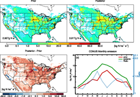
Figure 2. Spatial distribution of prior (a) and posterior (b) annual anthropogenic  emissions; (c) difference between posterior and prior annual anthropogenic
  emissions; (d) prior (red solid) and posterior (green solid) monthly anthropogenic
  emission for contiguous US, ratio of posterior/prior (blue dotted line).
Download figure:
Standard image High-resolution imageFigure 2(d) shows that total posterior anthropogenic  emissions peak in summer and have a similar seasonal pattern as the prior emissions, but increased significantly throughout the whole year by a factor of 1.1 to 1.6, especially during warm months, despite small-scale decreases (figure S3) in the Central Valley and southeast North Carolina, as well as in Northwest Iowa and southwest Minnesota from March to October. The largest percentage increase (about 64%) was found in May, strongly suggesting large underestimates in agricultural activities and emission factors.
Combining spatial distributions of  emission from different animal types based on Carnegie Mellon University's livestock emission model (U.S. EPA 2018) and spatial and temporal distribution of fertilizer application rate from Cao et al (2018), as well as figure 2(c) and figure S3, we can roughly conclude which sources of
  emissions might be biased in the prior inventory. The substantial underestimates over the central US (South Dakota, Nebraska, southwestern Kansas, northern Texas, and southern Wisconsin) and the northwestern US in spring are most likely due to underestimate of fertilizer use and manure application. The underestimate in northeastern Colorado and northern Texas during most of the year is likely caused by underestimated cattle emissions, consistent with previous studies (Battye et al 2016, Kille et al 2017) based on aircraft, ground, and satellite measurements. The moderate underestimate over most of the southeastern US is more likely due to poultry emissions, whereas the underestimate over southeastern North Carolina is more likely due to swine emissions. For southeastern Pennsylvania, the underestimate might be due to an underestimate of both livestock (swine and poultry) and fertilizer emissions during warm months. For the Delmarva peninsula area, the year-round underestimate is more likely caused by low emission factors of broiler chicken emissions (Russ and Schaeffer 2017).
While increases in  emissions occur over most of the domain, persistent decreases are found during warm months in a few areas (e.g. the Central Valley, northwest Iowa and southwest Minnesota, as well as Clinton and Duplin) with the densest cattle or swine population. These heterogeneous adjustments of
  emissions might be caused by 1) biased emission factors due to lack of differentiation in animal size and age, pasture and feedlot cattle, and manure management techniques (Battye et al 2019), and 2) the potential underestimation of CrIS
  over very high-emission areas (Dammers et al 2017).
Table 1 compares our posterior  emissions for the contiguous US in 2014 to previous bottom-up (European Commission 2011, Janssens-Maenhout et al 2015, Hoesly et al 2018, Crippa et al 2018) and top-down (Zhang et al 2012, Paulot et al 2014, Dammers et al 2019) studies. Our CrIS-derived annual
  emission estimate is 3.91 Tg N a−1, consistently higher than previous bottom-up estimates ranging from 2.4 to 3.40 Tg N a−1 and ground-based measurement derived estimates between 2.3 and 2.8 Tg N a−1. The generally higher estimates derived from satellite observations are likely due to 1) its greater spatial coverage and detection of elevated concentrations above surface level in the
  profiles, and 2) the high bias (
 5% for most values, but > 30% for small values) in CrIS
  concentrations (Dammers et al 2017). The difference between our estimate (1.3 times higher than HTAP v2 estimate) and that also derived from CrIS by Dammers et al (2019) (2.9 times higher than HTAP v2 estimate), might be due to the fact that Dammers et al (2019) used time-constant emission profiles for large point sources, targeted the years 2013 to 2017 while we only target the year 2014 which has lower CrIS
  concentrations compared to other years (Shephard et al 2020), used several estimated constant lifetimes (average of 2.35 h), and did not remove the influence of the CrIS retrieval a priori
  information. With proper diurnal emission profiles, top-down estimate from Dammers et al (2019) could be reduced by a factor of 2.0, which is 1.45 times higher than HTAP v2 estimate and much closer to our top-down estimate (1.3 times higher than HTAP v2 estimate) (Dammers 2020). For our 4D-Var inversion, application of averaging kernels has a larger impact on top-down
  emissions than diurnal variability of livestock emissions (see figure S5(a)).
Compared to previous top-down (Gilliland et al 2006, Henze et al 2009, Zhang et al 2012, Zhu et al 2013, Paulot et al 2014) and bottom-up (Pinder et al 2006, Cooter et al 2012, Paulot et al 2014, Janssens-Maenhout et al 2015) estimates, our posterior monthly emissions have similar summer/winter contrast, but generally higher magnitudes during most of the year except April, May and July. Our posterior estimates for mid-late spring (April and May) and July are lower than those from Gilliland et al (2006) based on NADP wet  , and Zhu et al (2013) based on TES
  , respectively. The largest difference among these monthly estimates lies in the spring/summer contrast. Wet
  -based emissions (Gilliland et al 2006, Pinder et al 2006, Paulot et al 2014) are generally higher in spring than in summer likely due to most of the NADP-wet
  monitoring sites being more representative of agricultural land cover (Bigelow et al 2001) where fertilizer use and manure application peak in spring, while satellite
  -based estimates, such as Zhu et al (2013) and our study, are always higher in summer likely due to the satellite's more uniform spatial coverage that captures the agricultural emission increases (both in livestock and fertilizer use) driven by increasing ambient temperature throughout the domain (figures 1(d) and (g)). Meanwhile, in-situ measurement-based inversions are prone to underestimating small but widespread
  emissions due to the sparsity of monitoring sites. The data filtering (retaining only pixels with Quality Flag of 5) in our inversion and the averaged 15% high bias in CrIS
  retrieval over the US compared to AMoN measurements (Kharol et al 2018) might also contribute to our generally higher posterior
  emissions, especially over the East US.
To further evaluate our CrIS-derived  emissions, we next compare prior and posterior simulated surface
  and wet
  concentrations against measurements from the AMoN, NADP, and SEARCH monitoring networks. For AMoN sites, we filtered out those sites with monthly mean beyond the monthly domain average by three times the standard deviation.
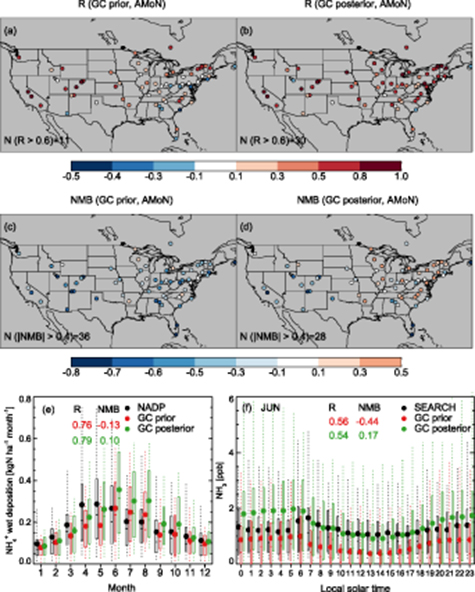
Correlation coefficients between time series of monthly mean GC surface concentrations and AMoN  measurements in 2014 for each site before and after emission optimization, respectively, are shown in figures 3(a) and (b). GC prior generally captures the spatial pattern (R between 0.51 and 0.81 throughout the whole year except February, figure S4) and seasonal variability in AMoN
  , but only 11 out of 65 sites had a correlation coefficient greater than 0.6. Ten sites (AZ98, FL11, GA40, GA41, MD99, NS01, NY96, OH02, SC05, WV18) have R less than -0.1. Most of these ten sites are located where
  emissions are small (less than 5 kg N ha−1 a−1, see figure 2(a)). Emission optimization enables the model to better reproduce the observed seasonal variability, increasing the number of sites with R greater than 0.6 to 30 and further leading to a moderate increase (from 0.53 to 0.84) in R between domain average monthly mean GC and AMoN measurements.
Figure 3. (a) Correlation coefficient between prior monthly mean GC surface  and monthly mean AMoN
  measurements; (b) posterior correlation coefficient; (c) normalized mean bias of prior annual mean GC surface
  relative to annual mean AMoN
  measurements; (d) posterior normalized mean bias; (e) Boxplot of monthly mean of GC prior and GC posterior
  wet deposition, as well as NADP
  wet deposition; (f) Boxplot of hourly mean of GC prior and GC posterior surface
  , as well as SEARCH
  in June.
Download figure:
Standard image High-resolution image
Figures 3(c) and (d) show the normalized mean bias of annual mean GC surface  relative to AMoN
  measurements for each site. Low bias is found in the annual mean GC prior at most sites. 36 of 65 sites have NMB magnitude greater than 0.4. Emission optimization largely reduces the low bias for most sites at the annual scale, leading to an approximately three-fold decrease in domain NMB (from -0.45 to -0.16) at the annual scale. The number of sites with NMB magnitude greater than 0.4 is reduced to 28. Moreover, the magnitude of posterior monthly domain NMB is also reduced by a factor between 1.4 and 12.7 throughout the year except November (see figure S4).
Similar but less significant improvement is found in comparison with domain average monthly mean NADP wet deposition of  in 2014 (figure 3(e)). GC-simulated
  wet deposition consists of wet deposition of aerosol-phase
  and gas-phase
  . To remove the bias caused by the difference between measured and simulated precipitation, we scaled the measured wet
  by the ratio of modeled and measured precipitation, NADP wet
  × (Pmodel/PNADP)0.6, following Paulot et al (2014). We only compared simulated wet
  to measurements with Pmodel/PNADP between 0.25 and 4.0 (Paulot et al 2014). NADP-measured
  wet deposition is higher in warm months and peaks in spring, likely due to intense fertilizer and manure application. GC prior can capture the general summer/winter contrast but underestimates the magnitude during most of the year, especially in spring. Our CrIS-derived
  emissions improve the overall ability of the model to reproduce NADP wet measurements with a slight increase in R (from 0.76 to 0.79) and a slight decrease in NMB magnitude (from -0.13 to 0.10), although GC posterior still misses the springtime peak. The maximum percentage increase in anthropogenic emissions in the spring (figure 2(d)) is consistent with the higher springtime emissions reflected by NADP wet
  .
.
Figure 3(f) shows another evaluation using hourly measurements of surface  collected from five SEARCH sites (BHM, CTR, JST, OLF, YRK) in June 2014. While having a similar diurnal cycle as GC prior, GC posterior better reproduces the magnitude of monthly-averaged hourly SEARCH
  , reducing the NMB from −0.44 to 0.17 in June. A substantial decrease from -0.38 to 0.03 in NMB is found at the annual scale.
5. Discussion and conclusions
This study presents the first 4D-Var inversion of  using CrIS measurements. CrIS-derived monthly
  emissions are higher than HTAP v2 emissions across most of the contiguous US and throughout most of the year, despite occasional small decreases (
 40%), revealing a substantial underestimate of
  emissions from springtime fertilizer and manure application over the central US and widespread underestimation of total agricultural
  emissions (fertilizer + manure) associated with warm temperature.
New CrIS observations since 2018 (Glumb et al 2018) could help future studies constrain long-term  trends. We also emphasize that use of an observation operator (which contains critical information about the instrument's sensitivity to
  ) is critical for making comparisons between model simulations and CrIS
  profiles. For example, without consideration of the observation operator the difference between simulations and CrIS observations at surface level over polluted areas in July 2014 is three times higher than when using the observation operator (see figure S5 (a)), and commensurate differences could be expected in top-down emission estimates.
Given the critical role of  in
in  formation and excessive deposition of Nr, evaluation of
  emission is important for environmental policy. A series of
  emission control policies have been implemented in Europe (Giannakis et al 2019). However,
  emissions in the US have not been regulated for multiple reasons, one of which is the difficulty of emission monitoring (United States Department of Agriculture 2014). Top-down
  emissions at high spatial resolution (0.25
 ) derived from CrIS observations may provide future policy makers quantitative support for monitoring changes in
  emissions.
Acknowledgments
This study is supported by NASA 80NSSC18K0689. We acknowledge the National Atmospheric Deposition Program (NADP) for providing surface  (available at http://nadp.slh.wisc.edu/amon/) and wet
  measurements (available at http://nadp.slh.wisc.edu/NTN/). We acknowledge the SouthEastern Aerosol Research and Characterization Network (SEARCH) for providing hourly measurements of surface NH3 (available at https://10.412 1/uuid:d9ac07c4-2041-4241-8635-3838c657a6ff). We thank Jesse Bash and Venkatesh Rao (U.S. EPA) for useful discussions. The CrIS CPFR Version 1.5 ammonia data for 2014 is publicly available from Environment and Climate Change Canada (ECCC) (https://hpfx.collab.science.gc.ca/mas001/satellite_ext/cris/snpp/nh3/v1_5/global/2014/). GEOS-Chem adjoint v35m source code is available online (http://wiki.seas.harvard.edu/geos-chem/index.php/GEOS-Chem_Adjoint).