


Abstract
The Paris Agreement of the United Nation Framework Convention on Climate Change calls for a balance of anthropogenic greenhouse emissions and removals in the latter part of this century. Mexico indicated in its Intended Nationally Determined Contribution and its Climate Change Mid-Century Strategy that the land sector will contribute to meeting GHG emission reduction goals. Since 2012, the Mexican government through its National Forestry Commission, with international financial and technical support, has been developing carbon dynamics models to explore climate change mitigation options in the forest sector. Following a systems approach, here we assess the biophysical mitigation potential of forest ecosystems, harvested wood products and their substitution benefits (i.e. the change in emissions resulting from substitution of wood for more emissions-intensive products and fossil fuels), for policy alternatives considered by the Mexican government, such as a net zero deforestation rate and sustainable forest management. We used available analytical frameworks (Carbon Budget Model of the Canadian Forest Sector and a harvested wood products model), parameterized with local input data in two contrasting Mexican states. Using information from the National Forest Monitoring System (e.g. forest inventories, remote sensing, disturbance data), we demonstrate that activities aimed at reaching a net-zero deforestation rate can yield significant CO2e mitigation benefits by 2030 and 2050 relative to a baseline scenario ('business as usual'), but if combined with increasing forest harvest to produce long-lived products and substitute more energy-intensive materials, emissions reductions could also provide other co-benefits (e.g. jobs, illegal logging reduction). We concluded that the relative impact of mitigation activities is locally dependent, suggesting that mitigation strategies should be designed and implemented at sub-national scales. We were also encouraged about the ability of the modeling framework to effectively use Mexico's data, and showed the need to include multiple sectors and types of collaborators (scientific and policy-maker communities) to design more comprehensive portfolios for climate change mitigation.
Export citation and abstract BibTeX RIS

Original content from this work may be used under the terms of the Creative Commons Attribution 3.0 licence.
Any further distribution of this work must maintain attribution to the author(s) and the title of the work, journal citation and DOI.
1. Introduction
Mexico consumes the most fossil fuels of all Latin American countries (IEA 2016), contributing about 1.4% of total global greenhouse gas emissions (GHG) (INECC-SEMARNAT 2015). The government of Mexico has proposed actions to monitor and reduce its net GHG emissions to the atmosphere. In 2012, Mexico established a comprehensive General Climate Change Law (DOF 2012), which mandated the design and implementation of a national-scale monitoring, reporting and verification (MRV) system. In 2015 Mexico submitted its Intended Nationally Determined Contribution (INDC) to reduce GHG and Short-Lived Climate Pollutant emissions 22% by 2030, and 50% by 2050 relative to its emissions in 2000 (United Nation Framework Convention on Climate Change (UNFCCC) 2015), and further detailed the forest sector's contribution in its mid-century strategy (SEMARNAT-INECC 2016).
Mexico ranks twelfth in the world in forest area (FAO 2015). The Land Use, Land-Use Change and Forestry (LULUCF) sector is likely to be a net GHG sink of 140.6 Tg CO2e (INECC-SEMARNAT 2015, Skutsch et al 2017), compensating for one-fifth of the GHG emissions reported from all other sectors in 2013. Currently, Mexico reports GHG emissions for the LULUCF sector using the stock-difference approach with emissions factors estimated from country-specific forest-plot measurements (CONAFOR 2014).
Carbon stock changes in forest systems result from multiple dynamic processes (e.g. growth and mortality of biomass, litter production, decomposition of dead organic matter, natural and anthropogenic disturbances), which interact from the scale of a tree to the entire landscape (Nabuurs et al 2007). Mexico recognizes the importance of reduced uncertainty in estimates using more complex methodologies such as carbon dynamics models for measuring, monitoring and projecting future GHG emissions (PRONAFOR 2014, SEMARNAT-INECC 2016). Models are powerful tools that allow the integration of information about land sector carbon dynamics and analysis at different spatial and temporal scales in a consistent manner (Kurz et al 2009, Pilli et al 2017). Models also improve the understanding of the mechanisms controlling carbon exchange between the atmosphere and vegetation (Birdsey et al 2013). Models can also be used to establish baselines and create scenarios for comparing and examining future impacts of different activities on carbon dynamics (e.g. management, land-use change, natural disturbances; Metsaranta et al 2010, IPCC 2011, Smyth et al 2014).
Since 2012, Mexico´s National Forestry Commission (CONAFOR), with international financial and technical support, started to modify and adapt available methods and modeling frameworks to estimate the role of Mexican forest ecosystems on GHG emissions/removals (Dai et al 2014, Olguin et al 2015, Mascorro et al 2015, Kurz et al 2016a). Building upon previous work coordinated by the Commission for Environmental Cooperation CEC, the Forest Services of the three North American countries have continued to advance the use of these analytical frameworks to evaluate the effects of human activities on future GHG emissions and removals. Related projects in the US (Dugan et al in review, this issue), Canada and a North-American synthesis paper are also in preparation.
The first objective of this paper is to present a biophysical assessment of several forest policy alternatives proposed by the Mexican government that could contribute to meeting GHG reductions goals, within two states identified as priority areas for the implementation of REDD+ activities (reducing emissions from deforestation and forest degradation and sustainable management practices) in forests under social tenure (CONAFOR 2013, CONAFOR 2015). Earlier studies have identified that forest management practices and conservation can play a key role to mitigate climate change in Mexico (Masera 1995, de Jong et al 1997, 2007, Olguin et al 2011, 2016). Forest mitigation strategies should minimize net GHG emissions without compromising other societal needs (e.g. timber, fiber, energy, etc.) because changes in wood supply can affect the use of more emissions-intensive materials such as fossil fuels, concrete, and steel (Sathre and O'Connor 2010, Garcia et al 2015, Smyth et al 2016). We do not try to determine how specific policy outcomes such as reducing deforestation can be achieved, but instead seek to quantify the consequences of different mitigation scenarios for GHG emissions and removals. Our second objective is to share lessons learned from the use of the analytical framework to assess and rank alternative mitigation options that can help the policy-making community in Mexico and in other countries to prioritize mitigation actions, based on a systems-based approach which includes carbon dynamics in forests, carbon storage in harvested wood products (HWP) and changes in emissions from displacing emissions intensive products and fossil energy sources (Nabuurs et al 2007, Lemprière et al 2013, Kurz et al 2016b). This is the first comprehensive forest sector biophysical mitigation analysis using the same primary data employed in Mexico´s current MRV system. Analyses of economic costs of mitigation portfolios (Lemprière et al 2017) and of other socio-economic indicators (Xu et al 2017) can be conducted with the suite of tools used here linked with other types of assessment models, but because of the lack of data are well beyond the scope of this paper.
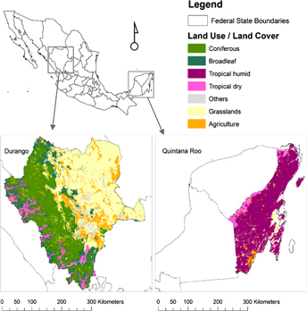
Figure 1. Durango (DGO) and Quintana Roo (QROO) study areas with main land-use/land-cover classes.
Download figure:
Standard image High-resolution image2. Methods
2.1. Study areas
In consultation with CONAFOR, we identified potential mitigation scenarios to evaluate in the states of Durango (DGO) and Quintana Roo (QROO) due to their sound institutional coordination of forest policy implementation and relevance of their forests for community-based management (Bray et al 2003, Garcia-Lopez 2013, Ellis et al 2015). These states provide contrasting biophysical characteristics, historic land-use changes, and contributions to national timber production (INEGI 2015a, 2015b). DGO (total area 12.3 Mha), containing principally coniferous forests, has had low historic rates of deforestation and produces a large volume of commercial timber. QROO (total area 4.4 Mha), in contrast, has had relatively higher rates of deforestation (twice that of DGO) in mainly tropical forest types with a low volume of timber production (figure 1). See supplementary information available at stacks.iop.org/ERL/13/035003/mmedia for detailed descriptions of study areas.
2.2. Modeling framework and data
We quantified the mitigation potential of the selected scenarios in the forest sector as the sum of the changes in net emissions, relative to a business as usual scenario. We used the Carbon Budget Model of the Canadian Forest Sector (CBM-CFS3) and the Carbon Budget Modelling Framework for Harvested Wood Products (CBM-FHWP). Both models are consistent with IPCC Guidelines for national GHG reporting (IPCC 2006). They have been adapted to represent Mexican conditions using data from Mexico. The scientific approach and necessary inputs for the parameterization of these models have been extensively documented in literature (Kurz et al 2009, Stinson et al 2011, Kull et al 2011, Pilli et al 2013, Smyth et al 2014, Kim et al 2016) and the supplemental material. The CBM-CFS3 implements the Gain-Loss method of the IPCC to estimate annual GHG emissions and removals in forest ecosystems. The CBM-FHWP model receives input from the CBM-CFS3 and tracks the fate of carbon in harvested biomass converted to wood products for various categories, uses, and landfills. Finally, we also estimate substitution benefits such as GHG emission reductions obtained from the use of wood products and biomass for energy (Smyth et al 2016).
Previous studies with the CBM-CFS3 in Mexico used a spatially-referenced framework that stratifies the country into 94 units based on the intersection of the 32 federal states with seven ecoregions of the North America Level 1 classification (Olguin et al 2015). The two states used in this study included six of these 94 spatially-referenced units (figure S1). We compiled and harmonized data from national, state and municipal levels on: forest distribution and forest growth (from Mexico´s National Forest and Soil Inventory, CONAFOR 2012), rates of fires, commercial harvests and land-use changes, ecological parameters (e.g. litterfall and decomposition of dead organic matter), climate, and data on harvested wood products and displacement factors (i.e. the change in emissions resulting from substitution of wood for more emissions-intensive products and fossil fuels). We estimated forest GHG emissions and removals in annual times steps for the period 2000–2050.
2.3. Simulation scenarios
We constructed a business as usual (BAU) baseline scenario and 4 mitigation scenarios (with 2 sub-scenarios). The BAU baseline estimates the GHG fluxes if forest management and disturbance rates observed in the past continue into the future (2018–2050). We extended the average annual gross rates from the last 10 year period of available activity data for land-use change (LUC) (2000–2010) in ha/year, harvests (2005–2014) in m3 of wood/year and area burned (2007–2016) in ha/year. Net ecosystem CO2e balances for the two states were generated as the sum of all GHG emissions and removals corresponding to carbon transfers in above- and belowground biomass, dead wood, litter and mineral soil forest carbon pools. We also estimated the net emissions from HWP production and use in the BAU by assuming that neither changes in policies nor changes in forest carbon cycling would occur due to climate change.
We estimated the biophysical mitigation potential (relative to BAU) if, by 2030, the following activities would be fully implemented (table 1): (M1) net zero deforestation rate, resulted from the reduction of gross deforestation rate (conversion from forest land to non-forest land) to equal gross forest recovery rate (conversion from non-forest land to forest land), (M2) M1 plus 10% increased net forest recovery rate, and (M3) increased forest productivity and timber production. For M3, we examined four sub-scenarios resulting from changes in the HWP component: (i) increased harvest using the same commodity proportions as in BAU; (ii) the increased harvest volume directed entirely to long-lived products (LLP); (iii) avoiding GHG emissions from more emissions-intensive materials (substitution benefit) using low displacement factor values; and (iv) avoiding GHG emissions estimated with medium displacement factor values. The last scenario (M4), combines all the activities (M2 and M3, including sub-scenarios). In all cases, we simulated a linear transition from BAU in 2018 to the full implementation of the mitigation actions in 2030.
Table 1. Summary of the four mitigation strategies and sub-scenarios (relative to business as usual—BAU) for the forest ecosystem (FE), Harvested wood products (HWP) and substitution benefit (SB) components, in Durango (DGO) and Quintana Roo (QROO).
| Strategy name | Description | Parameter changed | Parameter value |
|---|---|---|---|
| M1. Net zero-deforestation | FE: Gradually reduce gross deforestation rate until in 2030 equals to gross recovery rate. It excludes forests within managed areas. | New gross deforestation rate (Kha yr−1, % reduction from BAU) a) DGO b) QROO | 3746 (−49%)7661 (−53%) |
| M2. Increased net forest recovery rate | FE: Same gross deforestation rate as in M1, but 10% more forest recovery rate from more intensified practices in non-forest lands. | New gross forest recovery rate (Kha yr−1, % increased from BAU) a) DGO b) QROO | 375 (+10%)766 (+10%) |
| M3. Better growth + more harvest + more HWPs with substitution benefits (4 sub-scenarios) | FE: Increased productivity and production in forests over a 50 year s rotation cycle, from improved thinnings, road infrastructure, fire and pest controls, within managed areas.HWP: (i) More carbon transferred but same proportion of commodities as in BAU or(ii) 100% of increased harvest goes to longer-lived products (LLP)SB: (iii) Low substitution benefit for wood products or(iv) medium substitution benefit | Forest area affected (ha)a a) DGO b) QROOAdditional annual harvest (t C yr−1, %) a) DGO b) QROOAdditional growth (m3ha−1yr−1)bIn sub-scenario (ii), sawn wood component changes in percentages points relative to BAU: a) DGO b) QROODisplacement factor for sawn wood—panels:Low (t C avoided/t C used)Medium (t C avoided/t C used) | 3 576 086507 429218 025 (+50%)6788 (+50%)2.7+9%+7%0.54–0.452 |
| M4. All forest strategies + more HWPs with substitution benefits | M2 and M3 combined (including sub-scenarios) | M2 and M3 combined (including sub-scenarios) |
aManaged areas map provided by CONAFOR and intersected with INEGI´s Land-use/Land-cover map, year 2011, reclassified into broad forest categories harmonized with Mexico´s Biennial Update Report (see SI). bIncreased growth was modeled from two measurement cycles from National Forest Inventory.
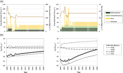
Figure 2. Annual CO2e balance in the states of DGO (left column) and QROO (right column) for the historic (2000–2017) and Business as Usual (2018–2050) periods. Panel (a) shows annual estimates of disturbance events, while panel (b) shows the effect of these disturbances on GHG emissions and removals by land-use category. Note that the scale of the Y axis for merchantable harvest in panel (a) is different for both states. FLFL: forest land remaining forest land, OLOL: non-forest lands remaining non-forest lands, FLOL: forest land converted to non-forest lands, OLFL: non-forest lands converted to forest land.
Download figure:
Standard image High-resolution image
Figure 3. Cumulative mitigation for four scenarios (with sub-subscenarios) in the states of DGO (left column) and QROO (right column) by component: (a) forests, (b) HWP, (c) displacement and (d) the total cumulative mitigation.
Download figure:
Standard image High-resolution image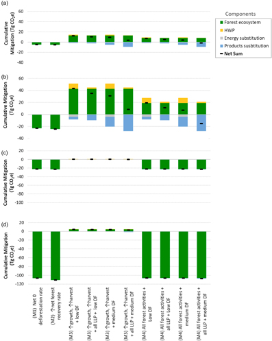
Figure 4. Cumulative mitigation for all systems components and scenarios for the states of DGO (a: year 2030, b: year 2050) and QROO (c: year 2030, d: year 2050).
Download figure:
Standard image High-resolution image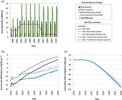
Figure 5. Comparison of BAU and scenarios M1 (net zero deforestation rate) and M2 (increased net forest recovery rate) in the forest ecosystem component of QROO, with (a) gross deforestation rates doubled and gross reforestation rates increased such that the net deforestation rate is the same in both scenarios (historic period only shown for clarity), (b) annual net GHG balance and (c) cumulative mitigation for M1 and M2 scenarios in the forest component.
Download figure:
Standard image High-resolution image
Net GHG emissions in all scenarios were calculated as the sum of the GHG fluxes in the forest ecosystem, HWPs and substitution benefit components. To assess the mitigation potential of the proposed strategies, we subtracted from each mitigation scenario the net GHG emissions of BAU, and reported both annual and cumulative emission reductions to 2030 and 2050 at the state level. Net emissions before 2018 were identical for all scenarios as estimated in the BAU baseline.
2.4. Land-use change (LUC) analysis
The relatively coarse spatial and temporal resolution in the available land-use/land-cover maps (i.e. four- to nine-year periods, 25 ha minimum mapping unit) could lead to the underestimation of gross deforestation and forest recovery rates (Mascorro et al 2015). Thus, as a sensitivity analysis, gross deforestation rates were doubled (in ha deforested per year) and gross forest recovery rates increased (ha/year) such that the net deforestation rate remained the same in BAU and in mitigation scenarios to assess the possible impact of underestimating the gross conversion rates of forest land to other land uses.
3. Results
3.1. Historic and baseline emissions
Activity data. The historic and projected deforestation and forest recovery areas for the period 2000–2050 are shown in figure 2(a) for DGO (left) and QROO (right). In the historic period, rates of deforestation in DGO are low but variable, while forest recovery remained at a relatively stable rate. In QROO, the deforestation rate was relatively constant while forest recovery was more variable and both rates were much higher than in DGO.
The municipal level data on area burned are highly variable in both states. DGO has a minimum annual area burned of 615 ha yr−1 and a maximum of 51 755 ha yr−1. The mean of 18 711 ha yr−1 is projected into the future for the baseline, despite the high standard deviation (±17 230 ha yr−1). QROO had corresponding values of 447 ha yr−1 and 79 161 ha yr−1 for the minimum and maximum annual area burned, respectively, and a mean of 18 083 ha yr−1 with a standard deviation of ±22 077 ha yr−1 (figure 2(a)).
Harvest rates in DGO are almost an order of magnitude greater than in QROO (figure 2(a)). DGO produces nearly 1/3 of all harvested wood (mean 436 051 Mg C yr−1) recorded in Mexico's national statistics with the variability in production driven by economic conditions (SEMARNAT 2014).
Emissions. Both states were estimated to be net sinks throughout the analysis period (figure 2(b)): 2000 to 2050. QROO was a sink of −14.1 Tg CO2e yr−1 compared to −7.96 Tg CO2e yr−1 for DGO. The contribution of different land categories varied with the strongest sink in forest land remaining forest land (FLFL).
Net GHG emissions in FLFL respond to (1) forest age structure which drives overall uptake rates by forest type, (2) emissions from forest fires and harvests, and (3) changes in forest area. Both states are strong sinks in the historic period (2000−2017), mean −9.7 and −17.7 Tg CO2e yr−1 in DGO and QROO, respectively. The sink strength in both states decreased over time in the baseline estimates: in DGO from −8.7 Tg CO2e in 2017 to −6.1 Tg CO2e in 2050 and QROO from −15.9 Tg CO2e in 2017 to −8.0 Tg CO2e in 2050; due to forest ageing and continuous reduction in forest area. The faster growing, relatively younger forests of QROO were a stronger sink in the historic period and at the beginning of the baseline, but they approach the sink strength of the forests in DGO by 2050. The variability seen in the historic period arises from varying incidences of disturbances, with reductions in sink strength corresponding to years with high rates of fires and harvests. This variability is removed in the projections because we use average annual fire and harvest rates in the BAU (figure 2(b)) and mitigation scenarios.
For forest land converted to other land (FLOL) during the historic period, emissions vary with the gross deforestation rates. FLOL emissions throughout the historic and baseline periods in DGO are low (1.51 Tg CO2e yr−1) compared to QROO (5.91 Tg CO2e yr−1). Both states show increasing emissions as more lands are deforested. The CBM-CFS3 simulates decay of wood residues over time and thus emissions increase as cumulative FLOL area increases. Forest recovery (OLFL) contributes a weak sink in DGO (−0.381 Tg CO2e yr−1) and QROO (−1.57 Tg CO2e yr−1) strengthening slightly over time as recovered forest area is added. Non-forest land (OLOL) emissions are shown here for completeness and represent small emissions on lands deforested more than 20 years ago. This analysis does not include emissions from land use of non-forest lands.
3.2. Mitigation
The cumulative mitigation benefits are summarized for forest, HWP and substitution (figure 3). Negative values represent an actual mitigation benefit, while positive numbers represent an increase in emissions with respect to the BAU scenario. In both states scenario M2 (net zero deforestation plus a 10% increase in forest recovery) achieved the greatest cumulative emissions reductions through 2050 of −24.4 Tg CO2e in DGO and −110.9 Tg CO2e in QROO. The greatest contribution within this scenario was achieved through a ∼50% reduction in gross deforestation rates relative to BAU, the same annual reduction reached in the net zero deforestation rate (M1 scenario). Thus, both M1 and M2 scenarios gave DGO a cumulative net emissions reduction of 2% in 2030 and 7% and 8%, respectively in 2050 (figure 3(d)). In QROO, the emissions reduction was 6% in M1 and M2 scenarios in 2030, and 23% and 24% respectively in 2050 (figure 3(d)). The more than threefold mitigation potential in 2050 of QROO compared to DGO is because QROO has greater changes in gross deforestation and forest recovery rates (table S2), as well as more rapid carbon accumulation rates and higher forest carbon density (figure S3, table S6).
Increasing forest productivity combined with increasing harvest rates (scenario M3) always yielded a relative increase in the forest emissions component relative to BAU because the increased C uptake is unable to offset the emissions associated with the greater increase in harvest (figure 3(b)). The managed forest area in QROO is relatively small and contributes only 0.6% to Mexico's annual harvest. Thus, even at year 2050, the cumulative carbon loss from increasing harvest rates is quite small in the M3 and M4 scenarios (figure 4(d)). In contrast in DGO, where more than half of the forest area is under silvicultural management, the carbon loss from harvesting 50% more and using the lower displacement factor (0.5 MgC avoided/ MgC wood used), generated 14% more CO2e emissions by 2050 relative to BAU (figure 4(b)). The cumulative mitigation benefit became positive, with a 4% emissions reduction relative to BAU, only when the increased harvest rate was combined with higher forest recovery rates as in M4 scenario, and all the extra carbon transferred to HWPs goes to sawn wood and we assumed a displacement factor of 2 MgC/MgC (figure 4(b)).
The average annual benefit varied by decade for the different mitigation scenarios (table 2). For both states, scenario M2 provided the most emissions reductions, however the rankings of other scenarios varied over time. The carbon losses in the M3 scenario decreased towards the end of the simulation (table 2). Had we assumed full implementation of this strategy earlier than 2030 (thereby increasing the number of harvest cycles of relatively fast-growing forest) the mitigation potential would have increased. These results show that the assumed increase in productivity does not offset potential C stock reductions resulting from increased harvest rates. While increases in forest productivity through forest management can be achieved, to maintain C stocks, the overall rates of harvests need to be limited if increasing forest C stocks is also a goal.
Table 2. Average annual mitigation (TgCO2e yr−1) by decadal range: 2021–2030 (A), 2031–2040 (B), and 2041–2050 (C), for each scenario and sub-scenario.
| Mitigation strategies | Durango | Quintana Roo | |||||
|---|---|---|---|---|---|---|---|
| A | B | C | A | B | C | ||
| M1. Net 0 deforestation rate | −0.46 | −0.85 | −0.98 | −2.14 | −3.88 | −4.55 | |
| M2. ↑ net forest recovery rate | −0.48 | −0.88 | −1.03 | −2.24 | −4.03 | −4.75 | |
| M3. ↑ growth and ↑ harvest | (i) + Low DF | 1.12 | 1.62 | 1.49 | −0.001 | 0.19 | 0.23 |
| (ii) + Low DF | 0.95 | 1.31 | 1.16 | −0.01 | 0.18 | 0.22 | |
| (i) + Medium DF | 0.83 | 1.16 | 1.03 | −0.01 | 0.17 | 0.21 | |
| (ii) + Medium DF | 0.31 | 0.33 | 0.18 | −0.03 | 0.14 | 0.18 | |
| M4. All forest strategies | (i) + Low DF | 0.67 | 0.72 | 0.49 | −2.13 | −3.87 | −4.52 |
| (ii) + Low DF | 0.50 | 0.42 | 0.17 | −2.14 | −3.88 | −4.53 | |
| (i) + Medium DF | 0.38 | 0.27 | 0.04 | −2.14 | −3.89 | −4.53 | |
| (ii) + Medium DF | −0.14 | −0.56 | −0.81 | −2.16 | −3.92 | −4.57 | |
Notes: (i) More carbon transferred but same proportion of commodities as in BAU, (ii) 100% of increased harvest goes to longer-lived products (LLP)
3.3. Sensitivity analysis of activity data
Maintaining the net deforestation rate but increasing the magnitudes of gross deforestation and forest recovery rates reduced the mitigation benefit in the M1 scenario because there are more emissions in the new BAU (e.g. −98.2 Tg CO2e in 2050). In contrast, under the M2 scenario, a 10% increase in the forest recovery rate yielded a 33% mitigation benefit relative to the new BAU by 2050 as more overall forest area was recovered (figure 5 (a)).
4. Discussion
This study provides initial assessments and lessons learned on the potential biophysical GHG impacts of the mitigation strategies outlined in Mexico´s NDC. Although beyond the scope of the current analyses, socio-economic analyses should be integrated with the biophysical models to understand potential barriers to implementation and the practical limits to deploying mitigation activities (e.g. Lemprière et al 2017, Xu et al 2017).
4.1. Regional variation in mitigation potential
National policies have different effects on actual emissions reductions depending on local forest characteristics and historic rates of LUC and it is therefore important to consider different policies at the state or even municipal levels when designing mitigation strategies. For example, a mitigation target based on a change of activity data (e.g. net zero deforestation rate) may yield similar types of benefits, but at very different magnitudes depending on where it is implemented. In this study, avoiding deforestation has significant mitigation benefits in QROO and much less so in DGO, because of the different deforestation rates in the baseline case and differences in forest carbon density at maturity (higher in QROO and lower in DGO).
4.2. Timing of policy implementation is important
In the case of DGO, if harvest is increased by 50%, it will generate higher CO2e emissions relative to BAU. However, implementing forest management actions sooner (e.g. transitioning sooner to higher productivity and harvest cycles) can ameliorate the increase in CO2e emissions in the M3 scenario by 2050 and provide other co-benefits such as increasing revenues from LLP and diversified job options. In addition, timing is also relevant for enhancing the mitigation potential of other strategies, such as increasing benefits from enhanced forest recovery (the earlier the better) or the duration of carbon stored in HWPs.
4.3. Interactions among mitigation activities changes the benefits over time
In the M4 scenario (where all forest strategies are combined), adding more LLP and changing the displacement factor from a low to a medium value in DGO, changed the mitigation potential so that M4 became the best mitigation scenario that included increased harvest for that state (last sub-scenario in figure 4(b)). Although more local data on displacement factors are required, this example shows the role that HWPs can play in achieving forest carbon mitigation targets and highlights the importance of including them in national GHG inventories.
4.4. Uncertainty about activity data may change the magnitude of the mitigation potential but not the ranking of scenarios
One of the key sources of uncertainty in assessing impacts of future scenarios was the rate of LUC. These data were derived from a change assessment over multi-year periods. However, given the length of the observation period and the high rates of forest growth, some areas may have had undetected forest cover loss and regrowth between observations. For example, Urquiza et al (2007) and Lawrence and Foster (2002) report that basal area of secondary forest stands (∼25 years old) in QROO, already had reached 40% of that of old-growth (>50 years old). If such disturbance/regrowth events occured between observations, then the gross rates of land-use changes would be higher than those assumed in our analyses.
New annual land-use/land-cover maps are being produced at various spatial and temporal resolutions (e.g. Hansen et al 2013, Gebhardt et al 2014/MAD-Mex system) and these could be used in the future to derive more accurate estimates of annual gross rates of LUC. Re-running the analyses for QROO using the higher gross LUC rates but same net deforestation rate (figure 5(a)) increased the estimate of GHG emissions, and reduced the size of the sink in the later years of the BAU and mitigation simulations (figure 5(b)). In the adjusted BAU (dotted black line), the cumulative CO2e sink is 23% lower (−46.7 TgCO2e) than the original BAU (solid black line). However, the differences in the cumulative mitigation benefits are quite small (figure 5(c)). While the available activity data (derived from relatively coarse spatial and temporal resolution) might be underestimating gross rates of LUC and therefore net CO2 emissions, the rank order of the mitigation strategies remains unchanged.
4.5. Crucial to consider a systems approach when assessing mitigation scenarios
Reducing gross deforestation could provide significant biophysical mitigation potential, particularly in QROO. Mexico´s Emissions Reduction Initiative (FCPF 2016) identifies several activities for QROO including improved silvopastoral/agroforestry systems, sustainable forest management, environmental services payments, and strengthening local regulations and governance. In Mexico and in other countries in Central America, community-based forest management and ecosystem services payments programs are among the most effective policy options for improving forest cover (Min-Venditti et al 2017). Forest management currently has little impact on emissions in QROO. However, if the area under management is increased greatly, the benefit would be twofold; it would help to reduce the overall rate of deforestation and avoid forest degradation through illegal logging practices (the last two not considered in this analysis). It could also increase the number of policy actions and co-benefits (Kapos et al 2012, Skutsch et al 2017), expand the collaboration with other sectors (e.g. HWP for the tourism architecture in the Maya Riviera, Sierra-Huelsz et al 2017) and still maintain the positive mitigation benefits within the state.
5. Conclusions
Mexico has a national forest inventory that allows for reporting changes in all carbon pools every five years as part of its MRV system. However, with the collaboration of the three forest services of North America, CEC and other government partners, we assessed, the impacts of the main drivers (forest growth, harvest, fire and land-use changes) of past and projected emissions as well as mitigation activity scenarios. This information can support the design of low-cost, high-benefit, forest sector interventions (Aguillón et al 2009) to help achieve mitigation goals (e.g. NDC).
Using a consistent and transparent systems approach for the forest sector, we parameterized available tools with data from Mexico (e.g. forest inventory, activity data, HWP) to quantify the GHG mitigation potential of specific actions that the government has identified as priorities to reach emission reduction goals, while co-existing with other forest management policies (e.g. increasing national-scale timber supply and productivity—ENAIPROS).
The results clearly show that if reducing GHG emissions is the main goal, avoiding deforestation and increasing recovery following deforestation (M1 and M2 scenarios) is the primary strategy to do so. In both states, the greatest reduction came from reducing deforestation although the magnitudes between them varied greatly due to differences in their baseline rates and forest carbon densities. Because GHG reduction goals interact with other socio-economic aspects (e.g. the need for employment, timber, etc.), the results from this analysis show a variety of policy actions available to meet societal needs and still reduce GHG emissions (e.g. increase harvest for manufacturing of long-lived products, use of mill residues for bioenergy, use of wood products instead of steel or concrete).
In Mexico, the systems approach to estimate the mitigation potential had not previously been used, but this paper demonstrates the utility of using existing modelling frameworks, parameterized with local data, for both reporting past trends and analyzing future scenarios. Previous studies have examined the mitigation potential of the forest sector in Mexico (Masera et al 1997, Aguillón et al 2009, Garcia et al 2015); however, our study provides some additional insights since it: (1) identifies and assesses the main drivers of GHG emissions (e.g. forest growth, land-use changes), (2) does not assume fixed future emissions in either BAU or mitigation scenarios, recognizing changes over time (in forest area, forests age, etc.), (3) uses the same data that are used for national official reporting to the UNFCCC, (4) tracks carbon in HWP (currently assumed in Mexico´s official reporting as instantly oxidized after harvest), (5) assesses the potential interaction with other sectors to reduce emissions, (6) provides specific information related to Mexico´s NDC and mid-century plans for 2030 and 2050 and (7) demonstrates the implication of non-carbon objectives (e.g. increasing timber production) on the forest sector that may affect the success of reaching mitigation targets.
While the estimates of emissions and removals can be improved (e.g. when more detailed information becomes available on land-use change, displacement factors, etc.), this framework can be expanded to other regions of Mexico and other more complex scenarios could be analyzed (e.g. forest degradation reduction, sustainable forest management), and ranked against alternative mitigation policies. This work provides a solid foundation for the continued evolution and improvement for implementing the systems approach to mitigation by the forest sector in Mexico and the results are also applicable to other countries with similar mitigation goals.
Acknowledgments
Funding for this research was provided by the Commission for Environmental Cooperation (CEC) as part of a tri-national project. We are especially grateful to Karen Richardson and her colleagues in CEC for providing invaluable coordination and administrative support. We thank the three North American Forest Services (National Forest Commission of Mexico–CONAFOR, Canadian Forest Service of Natural Resources Canada, and USDA Forest Service) and encouragement by the North American Forest Commission (NAFC), the SilvaCarbon program, Mexico´s National Institute of Ecology and Climate Change (INECC) and other experts for their technical support. Specifically, we thank Raúl Rodríguez, Germánico Galicia, Jesús Rangel, Oswaldo Carrillo, Claudia Octaviano, Gregorio, Ángeles Benedicto Vargas, Javier Corral, Vanessa Maldonado and Ken Lertzman for the valuable information and comments provided to our analyses. The authors also wish to thank the Government of Norway, the United Nations Development Program (UNDP) and the UN Food and Agriculture Organization (FAO) for their financial and coordination support in an earlier stage of this work through CONAFOR´s project: 'Reinforcing REDD+ and South-South Cooperation'. The views expressed in this study do not necessarily reflect the positions of the Government of Durango, the Government of Quintana Roo, or the Governments of Mexico, the US or Canada.