

Abstract
A well-known feature of the observed and simulated climate is enhanced land surface warming compared to the ocean. This difference in warming, frequently expressed as a ratio, is often contrasted between the observed record and climate model output as both an evaluation metric for climate models and as a global index used for climate change detection and attribution. Latest simulated estimates of the ratio use full global coverage and marine surface air temperature, making genuine comparisons with observations difficult, since global observed data sets typically use sea surface temperatures (SST) and have limited spatial coverage. We show that re-calculating simulated ratios using SST and limited spatial coverage (to resemble the observations) raises the ratio by ∼0.25. We also update the observed ratio using latest observations and we find a close convergence of observed and simulated ratios towards ∼1.6 for the 2000–2016 period accompanied by a decline in temporal variability. If we revise estimates of the likely range of ratios from climate models to account for the above factors, then our new observed ratio estimate is slightly less than the median of the GCM ensemble range (1.54–1.81).
Export citation and abstract BibTeX RIS

Original content from this work may be used under the terms of the Creative Commons Attribution 3.0 licence. Any further distribution of this work must maintain attribution to the author(s) and the title of the work, journal citation and DOI.
1. Introduction
Greater levels of temperature change over the land surface, compared to the ocean surface is a well-noted phenomenon of climate change (e.g. Lambert and Chiang 2007, Sutton et al 2007, Drost and Karoly 2012a, Drost et al 2012b, Byrne and O'Gorman 2013). Interest in the warming ratio (hereafter 'WR') reflects the importance of the phenomenon in both societal terms (i.e. the implications of mitigating and adapting to global temperature targets over land) and also in terms of the dynamical processes responsible for the WR under both transient climate change and climate equilibrium. Existing studies provide substantial assessments of the coupled ocean–atmosphere processes which appear to be responsible for the WR showing that whilst thermal inertia differences do contribute, the dominating mechanisms are related to boundary layer properties, humidity and surface processes (e.g. Sutton et al 2007, Joshi et al 2008b, Byrne and O'Gorman 2018). Recent studies have also described how the nature of the WR is different depending on the forcing agent and land surface properties (including stomatal responses to CO2 concentrations) (Sutton et al 2007, Joshi et al 2008b, Joshi and Gregory 2008a). Other work has shown evidence for a land–sea WR under paleo-climatic change (Schmittner et al 2011) whilst other work has identified processes constraining the WR (e.g. oceanic heat uptake; cloud feedbacks) (Lambert et al 2011, Sejas et al 2014).
Braganza et al (2003) and Braganza et al (2004) considered simple land-minus-ocean temperature differences (rather than a ratio) finding a rising trend in the observed land–ocean contrast well-captured by GCM simulations and attributable to anthropogenic forcing. Sutton et al (2007) diagnosed an observed WR of ∼2.0 using data for 1980–2004 noting lower simulated WR values. Lambert and Chiang (2007) report an observed land–sea contrast in temperature change, also for 1980–2004, of ∼1.55 or ∼1.76 obtained by regressing ocean and land temperatures (the two estimates reflecting which variable is assumed independent). More recently, using additional GCMs involved in the UN Intergovernmental Panel on Climate Change's 5th assessment report (IPCC AR-5), the likely value of the WR has been placed between 1.4 and 1.7 (Collins et al 2013) whilst Drost et al (2012b) derive an observed WR of between 1.39 and 1.69 for 1990–2010 and a simulated WR of 1.54 for the same period using CMIP3 GCMs.
In this study we extend estimates of the present day and recent period WR using two estimates of observed land surface air temperature (SAT) and a set of historically-forced GCM simulations. We also investigate the sensitivity of the simulated WR to the choice of sea surface temperatures (SST) or marine SAT. The implications (as yet unquantified) of interchanging between SST and marine SAT deserve attention, especially when seeking to make like-for-like GCM-to-observation comparisons of the WR, given that major global observed records use oceanic SST rather than marine SAT.
2. Data and methods
2.1. Observed data
For the diagnosis of the observed WR we use two gridded instrumental records of monthly temperature. The first, HadCRUT4, spans 1860–2016 and is a blended data set of land SAT and ocean SST (Morice et al 2012). Uncertainty estimates are supplied for HadCRUT4 via an ensemble-sampling approach and for the purpose of our study here we use the median data set of the ensemble results. The second observed data set is the land-only Berkley Earth SAT record, hereafter 'BE', spanning 1750–2015 (Rohde et al 2013). The two observed records are selected to provide a representation of the sensitivity of observed temperatures to both station inclusion and, importantly, differing gridding and homogenization algorithms over the land surface (see Rohde et al 2013 for a description of how the latter contrast with techniques used by other groups) so-called 'structural uncertainties' (Morice et al 2012). By selecting BE as the alternative land data set such differences are larger and so the sensitivity clearer than if other data sets were used which applied similar assemblage techniques to HadCRUT4 (e.g. NASA-GISTEMP).
2.2. GCM data
For diagnosis of the GCM WR we use data from 21 GCMs within the IPCC AR-5 CMIP5 archive (Taylor et al 2012). In order to match the time coverage of the observed data sets, for each GCM we use data from the CMIP5 'historic' experiments (forced with historical estimates of greenhouse gases, aerosols and natural forcing) up to the simulated year 2004 and thereafter we append data from each GCM's RCP4.5 experiment. Since we are focusing upon the GCM's comparison with the observed record, we do not use GCM data past 2016 in the analysis and therefore the choice of RCP experiment is of minimal importance, since the anthropogenic forcing divergence (between each RCP) does not dominate the simulated climate until later (Hawkins and Sutton 2009).
We use ensemble means of each GCM's historical and RCP4.5 simulations to create the SAT and SST temperature anomalies from which the simulated WRs are calculated, except when investigating the temporal variability of the WR. When investigating the temporal variability we use just one ensemble member per GCM to calculate the land and ocean warming anomalies in order to retain unforced variability that would be dampened by using an ensemble mean.
2.3. Calculation of WR
The WR is defined as the mean land temperature change, ΔTL, divided by the mean ocean temperature change, ΔTO. In calculating the mean over land and ocean, grid cells contributing either to ΔTL or ΔTO are first area-weighted and are designated land or ocean according to whether the land fraction in the grid cell is less than or greater than 50%. For all data (observations and GCMs) the WR is calculated for each month for the 1890–2016 period before an annual average WR is calculated. ΔTL and ΔTO are calculated with reference to their respective 1890–1920 climatological average which represents a period in which the anthropogenic forcing is small allowing us to diagnose the WR during rising levels of anthropogenic forcing, whilst also allowing for a reasonable spatial coverage of observations (more so than, say, 1850–1880). It is also consistent with previous investigations (Drost and Karoly 2012a).
Because the spatial coverage of the observed anomaly data sets are not consistent through time we follow the approach of Braganza et al (2003) and develop a fixed mask that excludes grid cells which do not have at least 40 years of data (a year defined as having at least 6 months data present in a given cell) from 1900 onwards (figure 1(a)). The resulting mask does not change through time and observed data coverage can vary within the mask's extent (so long as the grid cell meets the inclusion criteria). The sensitivity of global indices to coverage variability within the mask's extent has been shown to be low (Braganza et al 2003). The mask is applied to the observed data before integrating ΔTL and ΔTO and we calculate the GCM WR both with the mask applied ('masked') and without ('unmasked') in order to quantify the sensitivity of the WR to the coverage.

Figure 1. (a) The fixed mask applied to both observed and GCM data prior to composing land and ocean mean temperature changes. Black grid cells are excluded from the averaging. (b) Time series of the annual WR (low pass filtered at 10 years) for HadCRUT4 (dotted), BE (dashed) and mean of the CMIP5 GCMs (thick). GCM data in this plot are the masked SAT:SST series and shading indicates 16th and 84th percentiles of the component 21 GCM series (also time filtered).
Download figure:
Standard image High-resolution imageIn the case of the observed WR, ΔTO is always comprised of SST since the ocean element of HadCRUT4 is HadSST3 (Kennedy et al 2011a) and for the BE analysis we substitute HadCRUT4 data points over land only (with the Berkley Land Surface data). In the case of the GCM WR, however, we calculate WR both using SSTs over the ocean (hereafter 'GCM SAT:SST') and oceanic SAT ('GCM SAT:SAT') so that we can investigate the effect of variable choice upon the WR value.
3. Results
Annual WR series for the recent period, 1980–2016, are shown in figure 1(b). All series converge after the year 2000 and we discuss this convergence later. For the 1980–2016 period the observed HadCRUT4 and BE WR (note BE finishes 2015) is 1.45 and 1.62, respectively (see table 1 for mean values). To investigate the BE and HadCRUT4 contrast we plot land temperature anomalies for both in figure 2, but benchmarked to their respective 1951–1980 climatology which allows a comparison of the two series for the early and modern parts of the series. For the climatological 1890–1920 period, against which we calculate ΔTL for the WR calculation, figure 2 shows that BE is notably cooler than HadCRUT4, thus BE ΔTL will be larger than the corresponding anomalies for HadCRUT4. It is interesting to note that beyond 2000 there is a reverse in the differences with HadCRUT4 land temperature anomalies being slightly larger than BE. The effect of this divergence moderates somewhat the tendency for the BE WR to be greater than the HadCRUT4 WR (but the divergence is not large enough to completely offset the 1890–1920 difference).
Table 1. Mean annual WR for the full 1890–2016 analysis period and subset time slices. For GCMs, WR values are for the masked SAT:SST data. 'GCM Range' is the standard deviation of the 21 constituent GCM values in each time slice. For 2000–2016 the inter-annual standard deviation, σ, of the WR is also shown.
| GCM | 1890–2016 | 1980–2016 | 1980–1996 | 2000–2016 σ | |
|---|---|---|---|---|---|
| ACCESS1-3 | 1.10 | 0.91 | 1.34 | 1.69 | 0.40 |
| bcc-csm1-1 | 1.56 | 1.47 | 1.51 | 1.53 | 0.20 |
| CCSM4 | 1.52 | 1.51 | 1.58 | 1.65 | 0.14 |
| CMCC-CM | 1.69 | 1.85 | 1.87 | 1.86 | 0.23 |
| CNRM-CM5 | 1.60 | 1.38 | 1.50 | 1.61 | 0.22 |
| CSIRO-Mk3-6-0 | 1.33 | 1.27 | 1.53 | 1.74 | 0.30 |
| EC-EARTH | 1.52 | 1.76 | 1.79 | 1.80 | 0.13 |
| FGOALS-g2 | 1.48 | 1.70 | 1.67 | 1.66 | 0.18 |
| GFDL-CM3 | 1.80 | 1.39 | 1.51 | 1.62 | 0.17 |
| GISS-E2-H | 1.22 | 1.44 | 1.55 | 1.64 | 0.20 |
| GISS-E2-R | 1.69 | 1.45 | 1.58 | 1.69 | 0.13 |
| HadCM3 | 1.47 | 1.48 | 1.59 | 1.68 | 0.15 |
| HadGEM2-ES | 1.37 | 1.02 | 1.39 | 1.69 | 0.33 |
| inmcm4 | 1.90 | 1.88 | 1.83 | 1.76 | 0.22 |
| IPSL-CM5A-LR | 1.43 | 1.46 | 1.50 | 1.54 | 0.05 |
| IPSL-CM5A-MR | 1.32 | 1.34 | 1.43 | 1.51 | 0.13 |
| MIROC5 | 1.19 | 1.06 | 1.36 | 1.62 | 0.17 |
| MIROC-ESM | 1.27 | 1.13 | 1.39 | 1.65 | 0.15 |
| MPI-ESM-MR | 1.89 | 1.75 | 1.78 | 1.80 | 0.19 |
| MRI-CGCM3 | 1.51 | 2.34 | 2.13 | 1.95 | 0.21 |
| NorESM1-M | 1.40 | 1.42 | 1.60 | 1.71 | 0.21 |
| GCM Mean | 1.49 | 1.60 | 1.48 | 1.68 | 0.19 |
| GCM Range (stdev of 21 values) | 0.22 | 0.20 | 0.33 | 0.11 | |
| Observations | |||||
| HadCRUT4 | 1.32 | 1.45 | 1.28 | 1.61 | 0.18 |
| BE | 1.43 | 1.62 | 1.57 | 1.68 | 0.14 |
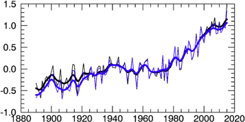
Figure 2. Annual land SAT anomalies (°C) for HadCRUT4 (black) and Berkley Earth (blue) with respect to their 1951–1980 means. Thick lines in each case are the 10 year low pass series.
Download figure:
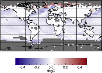
Standard image High-resolution imageFor the masked GCM SAT:SST data, which is the best resemblance to the observed data in terms of coverage and marine variable choice, the multi-model mean WR (1.60 for 1980–2016, table 1 and figure 1(b)) is very close to the observed values. By comparing the masked GCM SAT:SST and masked GCM SAT:SAT results we can quantify the sensitivity of the WR to marine variable choice. For 1980–2016 the masked GCM SAT:SST WR is higher than the masked GCM SAT:SAT WR (1.60 compared with 1.45). The larger simulated WR obtained when using marine SST instead of SAT can be attributed to lower warming of SSTs compared to SAT, with notable differences over the Northern Atlantic sub-polar gyre, the Sea of Japan and the Bering Sea (see figure 3). The regions of δSST and δSAT differences correspond with recently identified regions of increased oceanic heat uptake (Drijfhout et al 2014). The only region within the fixed mask where SST warms more than marine SAT is within the small number of Arctic cells that remain in the fixed mask (red, figure 3). Here, the replacement of sea ice by open ocean in winter months leads to a warmer simulated skin temperature and the skin warming associated with this phase change is much bigger than the local rise in SAT for the same time period. As expected, WR values calculated without the application of the fixed mask are lower due to the inclusion of Arctic oceanic grid cells which have substantial SST and marine SAT warming. The difference in WR for SAT:SAT due to the application of the mask is +0.09 and for SAT:SST it is +0.11. The magnitude of the masking affect is almost as large as the sensitivity of variable choice within the masked area. Accounting for both sensitivities, simulated WRs are approximately 0.25 higher for masked SAT:SST data than unmasked SAT:SAT, with the former being the best resemblance to the observations.
Figure 3. Multi-model mean differences between δSST and δSAT for the 1980–2015 period with reference to 1890–1920. Blue cells indicate SSTs have warmed less than SAT. Grey cells indicate the grid cells excluded from the WR calculation as per the fixed mask derived from HadCRUT4 observations.
Download figure:
Standard image High-resolution image
In all three data sources, HadCRUT4, BE and the multi-model mean (masked SAT:SST), a contrast in WR character during the recent 1980–2016 period appears evident before and after the year ∼2000 (table 1, final 3 columns and figure 1(b)). For the latter part of the recent period (after 2000) mean WR values converge towards very close agreement, with values of 1.61 (HadCRUT4), 1.68 (BE) and 1.68 (GCM multi-model mean). Simultaneously, for the 2000–2016 time period, a substantial reduction in the inter-model spread of WR values, measured by the standard deviation of the 21 simulated WR values, is evident compared to other time slices of the analysis period (e.g. an analogous 17 year period prior to 2000 (table 1 column 4, 1980–1996)).
The inter-annual standard deviation, σ, is calculated from the annual WR series for all data, for the 2000–2016 period in order to assess errors in WR in the period where well-mixed greenhouse gas (WMGHG) forcing is dominant (Joshi et al 2013). Values of σ prior to 2000 are sensitive to large fluctuations in WR arising solely from denominator values (ΔTO) being close to zero (for example, an inter-annual change in ΔTO of, say, 0.1, has a greatly amplified impact on WR variance than if ΔTO is 0 at t = 0 than, say, 1 at t = 0). In the case of the GCMs, WR from just one ensemble member is used to derive σ avoiding the suppression of unforced variability (which is present in the observations). For the 2000–2016 period the GCM multi-model mean σ (the mean of the 21 σ values, 0.19) is remarkably close to HadCRUT4 (0.18) and BE (0.14). For the observed 2000–2016 WR the standard error can be inferred ( ) giving respective uncertainty estimates of WR = 1.61 ± 0.09 for HadCRUT4 and WR = 1.68 ± 0.07 for BE. In the case of the simulated WR, in which there are 21 GCM series, uncertainty can also be estimated by the 16th and 84th percentiles of the 21 WR values. This choice of percentiles is equivalent to p = 0.66, and representative of the IPCC's 'likely' definition. By this definition, and by calculating percentiles in each year and then averaging those values for 2000–2016, the likely range of the simulated GCM WR is 1.54 to 1.81.
4. Discussion
The observed WR values for HadCRUT4 and BE for the recent period (1980–2016) agree well with previous calculations of the observed WR. Some previous studies have calculated higher observed WRs for example Sutton et al (2007) who calculated a mean value of ∼2.0 for 1980–2004. Suggestions have been made that discrepancies may exist between WR estimates made using observed records compiled before and after 2010 and that changes in the observation assemblage might account for higher values (Drost et al 2012b). Whilst bias corrections introduced into later records (most especially SST (Kennedy et al 2011a, Kennedy et al 2011b)) will influence the resulting WR and further corrections may still be required (Hausfather et al 2017) that could reduce the recent WR, we note in this study that there is sufficient sensitivity to the choice of reference period from which ΔTL and ΔTO are calculated to account for the large WR value of Sutton et al (2007). For example, the WR estimates in our study, (Drost and Karoly 2012a, Drost et al 2012b and Braganza et al 2003, Braganza et al 2004) all use a reference period of 1890–1920; if we re-calculate the observed WR in our study using ΔTL and ΔTO with respect to the 1961–1990 period, as per Sutton et al (2007) and Lambert et al (2011), then we arrive at a higher WR, 2.02 (HadCRUT4 for 1980–2004) which is commensurate with those studies.
Differences between the GCM SAT:SAT and GCM SAT:SST WRs show that WRs calculated using marine SAT are lower than if SST is used and that WRs are also lower if GCM data are not masked to resemble observational coverage. This behavior is consistent with recent investigations into simulated global-mean ΔT (Cowtan et al 2015, Richardson et al 2016) which is shown to reduce when coverage masking is imposed and, further, when marine SAT is substituted with SST thus influencing GCM comparisons against the observed global-mean temperature. It is important to also consider the differences in WR due to masking and variable choice when comparing observed WRs (of which all estimates, published to date, use SST) against simulated WRs where the variable choice over ocean is sometimes ambiguously described and may use unconstrained spatial coverage. The GCM sensitivity to oceanic variable choice, +0.15 in this study, and masking (a similar magnitude) will account for some of the reported discrepancies between observed and simulated WRs if the oceanic variable choices and spatial coverages are different.
The convergence of modelled and observed WR time series during the 1990s is consistent with the declining effect and changing spatial distribution of anthropogenic sulfate aerosols (Allen and Sherwood 2010). Prior to the 1990s aerosol forcing disproportionately cools the land, reducing the WR by an amount depending on aerosol forcing levels. Evidence for this lies in 1%/yr CO2 experiments, in which WR convergence occurs at much lower values of global temperature change than in historical-forced experiments (Joshi et al 2013). However, during the 1990s, the pattern of aerosol forcing shifts towards Eastern Asia and the Pacific Ocean (e.g. AeroCom Phase 2 emission data, Myhre et al 2013), and, consequently, is not concentrated over land as much as before, and therefore projects less on the WR. Such a shift is consistent with the results of Shindell et al (2015) who report a simulated WR from sulfate-only experiments during the period 1996–2005 which is similar in magnitude to WMGHG only studies: this period should be compared with our figure 1(b), which shows WR convergence during this period.
5. Conclusions
We have updated calculations of the WR index using the latest observed records and 21 historically-forced CMIP5 GCMs. We have shown that true like-for-like comparisons of the WR are sensitive to GCM oceanic variable choice and masking and that these sensitivities, ∼0.25 in total, will account for some discrepancies between observed and GCM WR comparisons. In order to isolate genuine differences (related to actual climate dynamics and processes) we propose that future comparisons take account of this. We have also shown sensitivity of the WR to the climatological benchmark from which land and sea temperature anomalies are calculated. Standardising future investigations to a common 1890–1920 reference period would better facilitate comparisons of WR between studies, at least those addressing the instrumental period.
Our results provide evidence to support the suggestion of the stabilization of the WR in recent years. We suggest that this stabilization is a consequence of: (i) emerging dominance of the WMGHG temperature response over aerosol forcing; (ii) changed aerosol distribution giving greater forcing over ocean compared to land; and (iii) progressive evolution in the size of ΔTO leading to a reduction in the noise of the WR series. The fact that WR estimates from observations and simulations are in very close agreement since the year 2000 suggests that the dynamical processes within the GCMs responsible for the land–sea warming contrast are responding realistically to well-mixed external forcing.
Acknowledgments
We acknowledge the World Climate Research Programme's Working Group on Coupled Modelling, which is responsible for CMIP, and we thank the climate modeling groups for producing and making available their model output and acknowledge the helpful comments of three anonymous reviewers of this manuscript. The authors were supported by UK NERC grant NE/N018486/1 'Robust Spatial Projections Of Real-World Climate Change'.