

Abstract
Albedo modification (AM) is sometimes characterized as a potential means of avoiding climate threshold responses, including large-scale ice sheet mass loss. Previous work has investigated the effects of AM on total sea-level rise over the present century, as well as AM's ability to reduce long-term (≫103 yr) contributions to sea-level rise from the Greenland Ice Sheet (GIS). These studies have broken new ground, but neglect important feedbacks in the GIS system, or are silent on AM's effectiveness over the short time scales that may be most relevant for decision-making (<103 yr). Here, we assess AM's ability to reduce GIS sea-level contributions over decades to centuries, using a simplified ice sheet model. We drive this model using a business-as-usual base temperature forcing scenario, as well as scenarios that reflect AM-induced temperature stabilization or temperature drawdown. Our model results suggest that (i) AM produces substantial near-term reductions in the rate of GIS-driven sea-level rise. However, (ii) sea-level rise contributions from the GIS continue after AM begins. These continued sea level rise contributions persist for decades to centuries after temperature stabilization and temperature drawdown begin, unless AM begins in the next few decades. Moreover, (iii) any regrowth of the GIS is delayed by decades or centuries after temperature drawdown begins, and is slow compared to pre-AM rates of mass loss. Combined with recent work that suggests AM would not prevent mass loss from the West Antarctic Ice Sheet, our results provide a nuanced picture of AM's possible effects on future sea-level rise.
Export citation and abstract BibTeX RIS
1. Introduction
A recent report from the US National Academy of Sciences 'recommends an albedo modification [(AM)] research program be developed' (NAS (US National Academy of Sciences) 2015). AM involves deliberately increasing Earth's reflectivity so as to avoid the surface air temperature increases associated with greenhouse gas emissions. AM belongs to a larger class of climate modification techniques that are sometimes called 'geoengineering.' The most commonly discussed AM technique involves lofting reflective particles into the upper atmosphere (Crutzen 2006). This form of AM is sometimes called solar radiation management (SRM; e.g. Keith et al 2010). Several studies argue that aerosol AM is relatively inexpensive (Barrett 2008, Robock et al 2009), and could be put into action quickly in the event of a 'climate emergency' (Keith et al 2010; compare Sillmann et al 2015). However, the uncertainties surrounding AM are large, and the risk of negative effects from AM is substantial (e.g. Robock et al 2009). The NAS report suggests that research into AM technologies is justified by the also-large risks posed by climate change.
The NAS report identifies sea-level rise as an impact of climate change, implying that AM could help avoid sea-level rise. An opinion piece by some of the NAS report's authors makes the link between AM and reduced sea-level rise more explicit; Keith et al (2010) suggest that technologies for AM should be developed for use in the event of climate emergencies, including large-scale ice sheet mass loss (compare Sillmann et al 2015).
The Greenland Ice Sheet (GIS) is sensitive to surface air temperature changes (e.g. Alley et al 2010), and might thus be a natural target for AM-based efforts to reduce sea-level rise. If all the ice presently stored in the GIS were to melt, sea level would rise by ∼7.3 m (Bamber et al 2013). The ice sheet's mass balance has become more negative during the last few decades (within large uncertainties; e.g., Rignot et al 2008, Sasgen et al 2012), in step with temperature increases (Vinther et al 2006). The GIS was smaller than today during past warm times and larger than today during past cold times (Alley et al 2010).
However, feedbacks in the GIS system may reduce AM's effectiveness in preventing mass loss from the GIS. The ice sheet's sensitivity to temperature change is a function of ice sheet size; ice sheets create their own local climates through their high elevations and reflective surfaces. If the GIS has partly melted when AM begins, its accumulation area will be reduced, possibly causing additional mass loss even after temperatures stabilize or begin to decline. Moreover, ice sheets grow more slowly than they shrink, because accumulation due to snowfall is slow compared to melting and calving. Consistent with these assertions, we have mapped out changes in the time scale of mass loss from the GIS with forcing temperature, reflecting the influence of feedbacks (Applegate et al 2014; see also Fyke 2011, Robinson et al 2012).
Sillmann et al (2015; see also Lenton et al 2008) argue that ice sheets may not give warning signs as they approach a 'tipping point,' and that preventing or reversing further ice mass loss once it has begun may require lowering temperatures below present-day values. Completely preventing melt from the present-day GIS might require lowering Greenland temperatures by ∼0.5 K (with large uncertainties), relative to the late 20th century (Applegate et al 2014). Preventing further mass loss after the ice sheet has already diminished in size would likely require even larger temperature reductions.
Moreover, one newly-published study indicates that AM would likely not prevent mass loss from the West Antarctic Ice Sheet (WAIS; McCusker et al 2015). Mass loss from the WAIS is driven by increased ocean temperatures, rather than the surface air temperature changes that drive changes in the GIS. In a series of experiments with a fully-coupled global climate model, McCusker et al (2015) found that AM did not prevent wind-driven delivery of warm water to the vulnerable margins of the WAIS. Thus, large sea level rise contributions from the WAIS may occur even under AM.
Despite the potential importance of AM as a method for avoiding the consequences of greenhouse gas emissions, relatively few studies have examined the effects of AM on the GIS in particular or sea-level rise in general. Here, we focus on two of these studies, Irvine et al (2009) and Moore et al (2010). Wigley (2006) and Irvine et al (2012) also simulate sea level rise under AM scenarios, but use treatments of ice sheet response and sea-level rise that are arguably simpler than those employed by Irvine et al (2009) and Moore et al (2010).
Irvine et al (2009) suggested that sea-level rise from the GIS could be eliminated by offsetting just 60% of the radiative forcing increase associated with a quadrupling of atmospheric CO2 concentrations using AM. To arrive at this conclusion, Irvine et al (2009) drove a model of ice sheet behavior to equilibrium over 104–105 yr using quasi-equilibrated climate model output.
Moore et al (2010) used a semi-empirical model of the relationship between radiative forcing and sea-level rise (Grinsted et al 2010, Jevrejeva et al 2010, 2012) to estimate sea-level rise up to 2100 given different emissions pathways and geoengineering methods. For scenarios in which the radiative forcing offset due to geoengineering grows rapidly with time, Moore et al (2010) found that sea-level rise might reverse after a few decades.
These earlier studies are groundbreaking, but neglect feedbacks that may be vital for proper assessment of AM's ability to reduce sea-level rise from the GIS. Irvine et al (2009) perform an idealized study in which they expose their simulated modern ice sheet to climate model-derived climatologies with increased atmospheric carbon dioxide concentrations and varying amounts of AM. However, they neglect the possibility that the ice sheet might already have lost mass by the time AM begins. Similarly, Moore et al (2010) use a single time scale for both sea-level rise and sea-level fall, implying that sea-level could be drawn down quickly. However, Grinsted et al (2010) noted that the true time scale of sea level adjustment is likely much longer for temperature decreases than increases. Thus, Irvine et al (2009) may overstate the effectiveness of AM in prevent sea-level rise from the GIS, whereas Moore et al (2010) may overestimate AM's ability to reverse sea-level rise once it has occurred. Moreover, Irvine et al (2009) examine the equilibrium response of the GIS, achieved over tens of thousands of years; however, decision-making requires consideration of sea-level change over decades to centuries.
Here, we investigate the response of the GIS to simple AM scenarios. We improve on previous work by using a three-dimensional model of the GIS (Greve et al 2011) that captures key feedbacks, and by focusing on the decadal to centennial time scales that are likely of greatest importance for decision-making. We also report modeled rates of GIS contributions to future sea-level rise, in addition to total GIS sea-level contributions.
2. Methods
To examine the potential effects of AM on the future development of the GIS, we drive an ice sheet model into the future using a variety of temperature forcing trajectories. One of these trajectories represents a no-AM case, whereas the others represent different AM scenarios. We then examine the differences in simulated ice volume losses and rates of ice volume change between the no-AM temperature trajectory and each of the AM scenarios (supplement4 ). Finally, we assess the potential effects of using a single time scale on semi-empirical model-based projections of sea level under AM scenarios (supplement).
Our base temperature forcing trajectory (black curves, figures 1(a) and (b)) is derived from a simulation with an Earth Model of Intermediate Complexity (EMIC; Schewe et al 2011) that follows the extended RCP8.5 emissions scenario (Meinshausen et al 2011). We used this EMIC run because it extends to the year 2500, but is broadly consistent with simulations using fully-coupled, high-resolution climate models in the CMIP5 ensemble that extend to 2300 (see results, below). Recent emissions follow RCP8.5 most closely of any of the Representative Concentration Pathways (Sanford et al 2014, their figure 1), suggesting that RCP8.5 is an appropriate 'business-as-usual' scenario (Riahi et al 2011; compare van Vuuren et al 2011). Moreover, AM is perhaps most likely to be deployed in higher emissions scenarios such as RCP8.5.
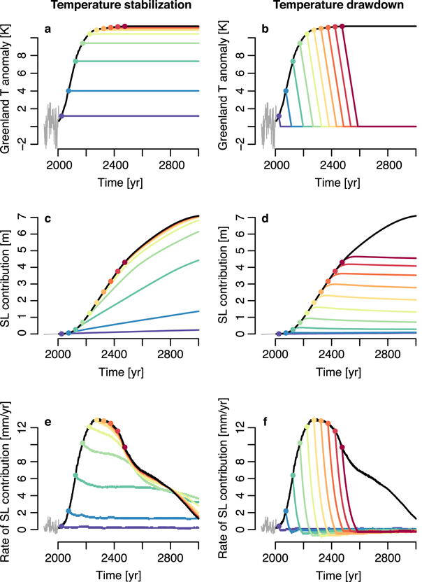
Figure 1. Temperature anomalies relative to 1976–2005 (a, b), simulated sea-level rise contributions (c–d), and simulated rates of sea-level rise contributions (e–f) over the period 1900–3000. Gray curves indicate the last 100 yr of model spinup, using temperature data from Vinther et al (2006). Black curves indicate the base, no-AM forcing trajectory. Colored curves indicate AM scenarios that diverge from the base scenario at 10 evenly-spaced dates between 2025 and 2475 (section 2); warm colors indicate later AM start dates (see table S1 for a color key). In the temperature stabilization scenarios (a), temperature anomalies level off at each of the branch points; in the temperature drawdown scenarios (b), temperature anomalies decline at 0.1 K yr−1 from each of the branch points until they reach 0. The no-AM case results in loss of the ice sheet by 3000 (c and d), as well as high rates of sea-level rise contributions (e and f). As expected, AM reduces total sea level contributions and rates of sea level contributions. T, temperature; SL, sea level.
Download figure:
Standard image High-resolution imageWe extracted Greenland-specific mean annual temperature anomalies relative to 1976–2005 from this climate model run by interpolating the gridded temperatures to the ice sheet model grid, then averaging over the interpolated values. We extended our temperature forcing scenario to the year 3000 by holding the temperature anomaly constant at its value in 2500. Although somewhat arbitrary, this procedure enables construction of a base temperature forcing scenario that is long enough to allow the ice sheet to adjust to the increased temperatures. Applegate et al (2014) suggest that the e-folding time for GIS adjustment to an 11 K temperature increase is ∼300 yr. Thus, driving the ice sheet model 1000 yr in the future (roughly three e-folding times) should allow the ice sheet adequate time to adjust.
We established 20 AM scenarios that diverge from the base temperature forcing trajectory (colored curves, figures 1(a) and (b)). The scenarios differ in terms of the year in which AM begins, as well as the 'style' of AM imposed. The AM scenarios diverge from the base scenario at 50 yr intervals between 2025 and 2475. The delay in imposing AM permits the ice sheet to partly adjust to changes in surface temperature, as required to evaluate the effects of feedbacks on the ice sheet's response to AM. In the temperature stabilization AM scenarios, temperature anomalies level off at whatever value they have reached when AM begins. In the temperature reduction scenarios, temperature anomalies decline from their pre-AM values to 0 at a constant rate of 0.1 K yr−1. This rate of temperature decline is high (Petschel-Held et al 1999), but is similar to the maximum rate of temperature rise in the base scenario.
3. Results
The base scenario (black curves, figures 1(a) and (b)) gives Greenland temperature increases of ∼4 K by the end of the present century and ∼11 K by 2300. These simulated temperature changes are quite comparable to mean Greenland temperature changes from the CMIP5 archive (Applegate et al 2014, their figure 4). Greenland warms about 40% more than the globe as a whole in this climate model simulation, also well within the range of results from CMIP5 (Applegate et al 2014, their figure 4).
Under the base scenario, the GIS disappears almost completely by the year 3000 (figures 1(c) and (d)). Total melting of the GIS in ∼1000 yr is rapid, but perhaps reasonable; based on a review of the then-existing literature, Lenton et al (2008) concluded that Greenland could achieve a 'largely ice-free state' in as little as 300 yr. The rate of GIS sea-level contribution under the base scenario increases to a peak value of ∼13 mm sle/yr around 2300 before declining to <2 mm sle/yr by the end of the millennium (sle, sea-level equivalent; figures 1(e) and (f)).
As expected, AM reduces total sea-level contributions and the rate of sea-level contributions from the GIS, relative to the base scenario (figures 1 and 2, S1–S3). The near-term effects of AM appear primarily as reductions in the rates of sea-level contributions from the GIS (figures 2(c) and (d), S3(e) and (f)). Depending on the style of AM and its start date, the reduction in these rates can be up to 12 mm sle/yr in the first century after AM begins. For comparison, present-day rates of sea-level rise from the GIS are ∼0.7 mm sle/yr, and the rate of total global mean sea-level rise is ∼3 mm yr−1 (Ablain et al 2009, van den Broeke et al 2009, Sasgen et al 2012). These rapid reductions in the rate of sea-level contributions disappear at later start dates for temperature stabilization AM, whereas they persist for temperature drawdown AM.

Figure 2. Reductions in total sea-level rise (a, b) and the rate of sea-level rise (c and d) in the first 500 yr after albedo modification begins, calculated as the difference between each of the AM scenarios and the base scenario. Gray areas indicate places where the value of interest becomes slightly negative. In general, AM produces relatively small reductions in total sea-level rise over the first century after AM begins, although these differences become large after several centuries (a and b). AM does produce appreciable reductions in the rate of sea-level change within the first few decades after AM begins (c and d). AM, albedo modification; SL, sea level; T, temperature; V, ice volume; m sle, meters of sea level equivalent.
Download figure:
Standard image High-resolution imageAM's effects on total sea-level rise from the GIS during the first few decades are considerably smaller than those that are realized over hundreds of years (figures 2, S1, S3; see also table S1). To take the most extreme case, beginning temperature stabilization AM in 2025 results in a reduction in total sea-level rise of ∼6.5 m by the end of the millennium (purple curve, figure S1(c)). However, the reduction in total sea-level rise is just ∼0.2 m (figure S3(c)) in the first century after AM begins. Thus, the near-term reduction in total sea-level rise under this AM scenario is ∼3% of the long-term reduction.
Importantly, for both temperature stabilization and temperature drawdown AM, sea-level contributions from the GIS continue after AM begins (figure 3). The one exception is the temperature decline scenario that begins in 2025, in which the ice sheet grows very slightly (<10−3 m sle) for a few decades before shrinking. The additional sea-level contributions from the GIS can be substantial, up to 1.2 m over the first century after the start of AM (figure 3). For temperature drawdown AM, sea-level rise from the GIS reaches a peak within ∼50–150 yr after AM begins, after which the ice sheet begins to regrow; however, the rate of regrowth is never larger than ∼1–2 mm yr−1 in our simulations (figure S3(f)).
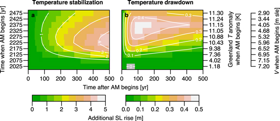
Figure 3. Additional sea-level rise as a function of AM start time and the time after AM begins, for both temperature stabilization (a) and temperature drawdown (b) AM scenarios. Note difference in scale between the two panels. Additional sea-level rise can be up to ∼1.2 m within the first century after AM begins, and grows to several meters after a few centuries for temperature stabilization. For temperature drawdown, additional sea-level rise reaches a maximum between ∼50 and ∼150 yr after AM begins, after which the ice sheet begins to regrow slowly. AM, albedo modification; SL, sea level; T, temperature; V, ice volume; m sle, meters of sea level equivalent.
Download figure:
Standard image High-resolution imageAfter tuning, the semi-empirical model used by Moore et al (2010; see also Grinsted et al 2010, Jevrejeva et al 2010, 2012) reproduces the ice volume losses projected by SICOPOLIS reasonably well in the base scenario (figure 4; supplement). However, the tuned semi-empirical model overestimates the reduction in sea level in the temperature decline scenarios, relative to SICOPOLIS. To take the most extreme case, if temperature drawdown AM begins in 2475 (red curves, figure 4), the tuned semi-empirical model projects a sea-level fall of ∼2 m by the end of the millennium, whereas SICOPOLIS estimates an additional sea-level rise of ∼0.3 m.

Figure 4. Simulated sea-level contributions from the Greenland Ice Sheet from SICOPOLIS (Greve 1997, 2005; solid lines) and a semi-empirical model (Grinsted et al 2010, Jevrejeva et al 2010; dashed lines). The semi-empirical model was tuned to reproduce the ice volume loss trajectory from SICOPOLIS in the base temperature trajectory (solid black curve) by minimizing the root mean squared error (supplement). The match between the solid and dashed black curves is acceptable; however, the results from the two models diverge strongly in the AM scenarios (colored curves), reflecting the lack of key feedbacks in the semi-empirical model. See table S1 for a color key. SL, sea level.
Download figure:
Standard image High-resolution imageThe parameter combination that we used throughout this study (black line, figure 5; supplement) simulates larger sea level rise contributions than any single model in the SeaRISE intercomparison project (Bindschadler et al 2013), including the SeaRISE ensemble member performed with the same model that we used (SICOPOLIS; Greve et al 2011). However, our preferred model run gives ice mass losses that are generally smaller than the other 'good' model runs in the same ensemble (blue lines, figure 5; Applegate et al 2012).

Figure 5. Comparison of the first 500 yr of the base scenario from the model run used in this study (black curve) to other ensemble members from Applegate et al (2012; blue and gray curves) and results from experiment R8 of the SeaRISE intercomparison project (Bindschadler et al 2013; colored dots). Blue curves, model runs from Applegate et al (2012) that yielded simulated modern ice volumes within 10% of the estimated value (7.3 m sea-level equivalent; Bamber et al 2013); gray curves, model runs from Applegate et al (2012) that yielded unreasonably large or small simulated modern ice volumes. The parameter combination used in this study (black curve; #29 from Applegate et al 2012) gives smaller mass losses than most other 'good' ensemble members from the same study (blue curves), but is more sensitive to temperature change than any model in the SeaRISE intercomparison project. See text for discussion. SL, sea level.
Download figure:
Standard image High-resolution image
4. Discussion
In this study, we used a simple ice sheet model to evaluate the ability of AM to reduce sea-level contributions from the GIS. Our results suggest that AM could produce substantial near-term reductions in the rate of sea-level rise due to GIS mass loss. However, our simulations also indicate that sea-level rise contributions from the GIS continue after AM begins, although these contributions are smaller than in a no-AM scenario. Even if surface air temperatures over Greenland are reduced rapidly through AM, regrowth of the ice sheet is slow compared to pre-AM rates of mass loss.
4.1. Differences between our study and Irvine et al (2009)
Irvine et al (2009) suggested that a partial offset of the radiative forcing associated with increased greenhouse gas concentrations would prevent sea-level rise from the GIS; in contrast, the GIS continues to shrink in all but one of our AM scenarios (figure 3). The two studies' findings likely diverge due to differences in (i) the range of temperature changes investigated in the two studies, and (ii) model initialization and the state of the GIS when geoengineering is begun.
Given that our AM scenarios generally start at higher temperatures than those investigated by Irvine et al (2009), it is not surprising that we find stronger ice sheet responses than they do. As noted above, Irvine et al (2009) created their no-geoengineering scenario by equilibrating a coupled climate model to a quadrupling of atmospheric carbon dioxide concentrations. In contrast, we used results from an intermediate-complexity climate model following the extended RCP8.5 scenario (Schewe et al 2011, Meinshausen et al 2011). These base scenarios imply different maximum radiative forcings (compare table 1 of Andrews et al 2012 with figure 4 of Meinshausen et al 2011), and therefore different maximum temperatures. Our base scenario levels off at a final temperature anomaly of ∼11 K, whereas Irvine et al (2009) found a maximum temperature increase over Greenland of ∼7 K, relative to the late 20th century (assuming that Greenland temperatures rose by about ∼1 K between the preindustrial period and the late 20th century; Vinther et al 2006). Moreover, because our AM scenarios diverge from the base scenario evenly in time, most of our AM scenarios achieve temperatures near the high end of our investigated range (figures 2 and 3; table S1); Irvine et al (2009) distributed their scenarios evenly in terms of radiative forcing, leading to an approximately-even distribution of their scenarios in temperature.
However, Irvine et al (2009)'s simulated ice sheet may be artificially insensitive to temperature change, because large ice sheets are less sensitive to temperature increases than small ones. Irvine et al (2009) equilibrate their ice sheet with the modern climate, as simulated by a coupled climate model. This procedure leads to a simulated modern ice sheet that is ∼18% larger, by volume, than the real ice sheet. In contrast, we selected the ensemble member that best matches the modern ice volume from an ensemble of 100 ice sheet model runs (Applegate et al 2012). Moreover, we allow the ice sheet to shrink in response to temperature rises before AM begins, whereas Irvine et al (2009) apply their equilibrated climate model output to the same initial GIS state in each case.
4.2. Evaluating the sensitivity of our model runs to temperature change
Our own model runs appear to be too sensitive when compared to the SeaRISE intercomparison project (Bindschadler et al 2013; figure 5), but not sensitive enough when the temperature threshold for ice sheet loss is considered. In our simulations, the GIS melts away completely given a sustained increase in local temperatures of 3–4 K, relative to late 20th century values (Applegate et al 2014, their figure 2(b)). This result implies that the GIS would eventually melt away if our temperature stabilization scenarios were maintained over many thousands of years, except for the scenario in which temperature stabilization begins in 2025. The temperature threshold values that we obtain are somewhat higher than those reported by Robinson et al (2012), who reported a threshold temperature of 0.8–2.2 K, assuming that Greenland has warmed by ∼1 K since the preindustrial period (Vinther et al 2006, their figure 10). Robinson et al (2012) present arguably the best estimate of the GIS' threshold temperature to date, due to their use of a relatively sophisticated surface mass balance model and careful calibration with geological data. Our ensemble agrees relatively well with mass balance estimates covering the last ∼60 yr (Rignot et al 2008, Applegate et al 2012, their figure 9). Thus, heuristic tests for assessing the sensitivity of our model runs are inconclusive.
In our opinion, the apparent discrepancy between our results and those of the SeaRISE intercomparison project is likely not due to our choice of ice volume as a metric for assessing the success of model spinup. This approach is clearly simplified compared to other proposed methods (supplement), but may represent an improvement over the method used to tune SICOPOLIS for the SeaRISE intercomparison project. Consistent with many prior ice sheet modeling studies, SICOPOLIS was tuned for the SeaRISE project by adjusting the model's input parameters one at a time to achieve a reasonable match to the observed ice thickness field. This procedure yielded a simulated modern ice sheet that is about 13% larger, by volume, than the observed ice sheet (Greve et al 2011, their figure 4(a)). Moreover, Chang et al (2014) used a Bayesian approach to show that there are multiple parameter combinations that give equally good representations of the modern ice thickness field. Adjusting model parameters by hand to achieve a reasonable match to observations is an informal gradient descent optimization method, which may become 'stuck' in local minima far from the optimal parameter combination (Chang et al 2014). Our method yields a simulated modern ice sheet with an approximately-correct ice volume by construction, and partly avoids problems with local minima by sampling evenly over a large parameter space.
4.3. Regrowth of the ice sheet in a semi-empirical model (Moore et al 2010)
After tuning, the semi-empirical model used by Moore et al (2010) reflects a much faster regrowth of the GIS than SICOPOLIS in our temperature drawdown scenarios (figure 4(b)). It should be noted that this semi-empirical model, as originally formulated by Grinsted et al (2010), applies to total sea level rise and is most appropriate for short-term projections (over ∼102 yr); here, we tune the semi-empirical model to represent the GIS component of sea level rise and extend its projections to the end of the millennium. This exercise is meant to demonstrate a particular limitation of the semi-empirical model used by Moore et al (2010), not to produce realistic projections of sea level change under AM scenarios. However, if the ice sheets make substantial contributions to future sea level rise, geoengineering may be less effective in reversing sea-level rise once it has already happened than Moore et al (2010) indicate.
4.4. Limitations and suggestions for future work
This study has several limitations that point to open research questions. As noted above, SICOPOLIS employs simplified treatments of ice flow and surface mass balance. We have partly examined this model structural uncertainty by comparing our model results to those from the SeaRISE intercomparison project (Bindschadler et al 2013; figure 5). In our experiments, temperature changes are simply added to the present-day climatology (Ettema et al 2010a, 2010b), and precipitation increases by ∼7% per degree of temperature increase (Greve et al 2011). This approach neglects potential spatial variability in future temperature changes, as well as the hydrologic responses associated with AM (e.g. Schmidt et al 2012). Also, our temperature trajectories do not incorporate interannual variability, which likely has an important effect on glaciers and ice sheets (e.g. Roe 2011). Proper incorporation of these effects would require a coupled climate-ice sheet model, as well as many more simulations.
As mentioned above, our no-AM temperature forcing trajectory is based on the extended RCP8.5 emissions scenario. Experiments using a similar methodology but lower emissions scenarios would likely show greater effectiveness of AM in either preventing sea level rise or helping the ice sheet to regrow, because the ice sheet would lose less mass before AM begins.
Moreover, the even distribution of our AM start dates between 2025 and 2475 means that most of our AM scenarios begin after 2100 (table S1). Further work might focus on earlier, and perhaps more policy-relevant, start dates for AM. Our existing model results suggest that early AM deployment produces larger long-term avoided sea level rise for temperature stabilization AM scenarios (though not temperature drawdown; figures 2(a) and (b)).
In this study, we have focused on the potential efficacy of AM in reducing sea level rise contributions from the GIS. The ice sheet is primarily sensitive to surface air temperature changes, and therefore would respond similarly to temperature changes caused by either AM or the reduction of greenhouse gas concentrations in the atmosphere. However, mitigation of emissions has a much slower effect on temperatures, and therefore might prove less effective than AM in reducing sea level rise.
4.5. Implications of this work
Despite the limitations of our modeling approach, our work helps provide a nuanced picture of AM's effectiveness in reducing GIS mass loss and sea-level rise. As pointed out by the recent US National Academy of Sciences report on AM (NAS (US National Academy of Sciences) 2015), sea level rise is an important consequence of climate change. However, using AM to prevent sea-level rise from the ice sheets (e.g. Keith et al 2010) may be less effective than intuition suggests, particularly over the first few decades after AM begins (figures 2(a), (b) and S3). Given that a recent climate modeling study suggests AM would not prevent mass loss from the West Antarctic Ice Sheet (McCusker et al 2015), this conclusion may apply to sea-level rise from the ice sheets generally.
Author contributions
KK initiated the study. KK and PJA designed the research. PJA carried out the model simulations, processed the model output, made the figures, and wrote the first draft of the manuscript. Both authors analyzed the model output and edited the paper text.
Acknowledgments
We thank Jacob Schewe for use of his CLIMBER-3α model output and Ralf Greve for providing his ice sheet model, SICOPOLIS, freely on the Web (sicopolis.greveweb.net). Nina Kirchner, Philipp Hancke, Martin Jakobsson, and Björn Eriksson provided computing resources at Stockholm University, Sweden. Peter Irvine and four anonymous reviewers provided helpful comments on drafts of this paper. This work was supported by the US Department of Energy, Office of Science, Biological and Environmental Research Program, Integrated Assessment Program, through grant DE-SC0005171; the National Science Foundation through the Network for Sustainable Climate Risk Mangement (SCRiM) under NSF cooperative agreement GEO-1240507; and the Penn State Center for Climate Risk Management. Some figure colors were drawn from www.colorbrewer.org by Cynthia Brewer at Pennsylvania State University. Table S1 was produced with tablesgenerator.com. All opinions and errors are ours.
Footnotes
- 4
The supplement contains additional information on our methods (sections S1.1–S1.4), table S1, and figures S1–S3, available at stacks.iop.org/erl/10/084018/mmedia. Our model output and code for generating the figures is archived on scrimhub.org.