

Abstract
Because the radiative forcing is rarely computed separately when performing climate model simulations, several alternative methods have been developed to estimate both the instantaneous (or direct) forcing and the adjusted forcing. The adjusted forcing accounts for the radiative impact arising from the adjustment of climate variables to the instantaneous forcing, independent of any surface warming. Using climate model experiments performed for CMIP5, we find the adjusted forcing for 4 × CO2 ranges from roughly 5.5–9 W m−2 in current models. This range is shown to be consistent between different methods of estimating the adjusted forcing. Decomposition using radiative kernels and offline double-call radiative transfer calculations indicates that the spread receives a substantial contribution (roughly 50%) from intermodel differences in the instantaneous component of the radiative forcing. Moreover, nearly all of the spread in adjusted forcing can be accounted for by differences in the instantaneous forcing and stratospheric adjustment, implying that tropospheric adjustments to CO2 play only a secondary role. This suggests that differences in modeling radiative transfer are responsible for substantial differences in the projected climate response and underscores the need to archive double-call radiative transfer calculations of the instantaneous forcing as a routine diagnostic.
Export citation and abstract BibTeX RIS

Content from this work may be used under the terms of the Creative Commons Attribution 3.0 licence. Any further distribution of this work must maintain attribution to the author(s) and the title of the work, journal citation and DOI.
1. Introduction
Radiative forcing quantifies the perturbation in radiative fluxes caused by changes in forcing agents. In addition to its instantaneous effect on the flow of radiation, a forcing agent can also cause changes in both the troposphere and stratosphere that further modify the upwelling radiative fluxes at the top-of-atmosphere (TOA). Because these changes occur independent of any change in global-mean surface temperature, they are generally classified as a component of the radiative forcing rather than a radiative feedback. This decoupling from the surface response also implies that radiative 'adjustments' to a forcing agent occur on a much shorter time-scale than radiative feedbacks and thus are also referred to as 'rapid adjustments'.
The cooling of the stratosphere in response to increased CO2 is the classical example of an adjustment to a forcing agent (Manabe and Wetherald 1967, Hansen et al 1981, 1997). The potential for cloud radiative properties to change in response to aerosol forcing has also been recognized for decades (e.g. Albrecht 1989, Penner et al 1992, Zelinka et al 2014). However more recent studies have identified the potential for clouds (and other tropospheric variables) to undergo rapid changes in response to CO2 forcing. It has also been noted that rapid adjustments to CO2 forcing are distinctly different from those to solar forcing (e.g. Andrews et al 2009, Bala et al 2010). Because these changes are believed to occur independent of changes in surface temperature, they have also been regarded as an adjustment to the forcing rather than as a feedback (e.g. Gregory et al 2004, Gregory and Webb 2008, Andrews et al 2009, 2012, Bala et al 2010, Colman and McAvaney 2011, Vial et al 2013, Zelinka et al 2013).
Recent studies have developed methods to infer radiative forcing indirectly using archived output from climate model simulations (Gregory et al 2004, Hansen et al 2005, Chung and Soden 2015). Based on these indirect calculations of forcing, several studies have found that differences in 'adjusted' radiative forcing introduce uncertainties in model projections of the climate response that are comparable to that resulting from the uncertainty in model-simulated climate sensitivity (e.g. Andrews et al 2012, Forster et al 2013, Vial et al 2013). These studies have identified cloud adjustments as the key contributor to the spread in adjusted forcing (e.g. Forster et al 2013, Zelinka et al 2013, Vial et al 2013, Ringer et al 2014). However, Chung and Soden (2015) have further suggested that a significant portion of the intermodel spread in adjusted forcing may actually result from differences in the instantaneous (or direct) forcing from CO2. We further investigate this issue by comparing estimates of radiative forcing for a quadrupling of CO2 using four different methods.
The instantaneous radiative forcing has been traditionally diagnosed by performing two sets of offline radiative transfer calculations for a limited set of atmospheric profiles (e.g. Collins et al 2006). Since these sets of 'double call' radiative transfer calculations are mostly performed separately from the actual climate model simulation which uses that forcing, it is difficult to compare explicit calculations of radiative forcing between models, even for the most idealized forcing scenarios.
Alternatively, Gregory et al (2004) developed a method for estimating the adjusted forcing by conducting a linear regression between global-mean surface temperature and TOA radiative fluxes from step-change CO2 experiments (i.e., the 'Gregory' method). Another alternate method for estimating the adjusted forcing (i.e., the 'Hansen' method) uses model simulations in which climate feedback processes are suppressed by prescribing sea surface temperatures (SSTs) while imposing an external forcing (e.g. Hansen et al 2005, Bala et al 2010, Held et al 2010, Forster et al 2013). However, it is not possible to separate the instantaneous forcing from the radiative adjustments using either the Gregory or Hansen methods.
Radiative kernels were developed to describe the differential response of TOA radiative fluxes to incremental changes in climate variables (Soden and Held 2006) and have become widely used to quantify the importance of different feedback processes (e.g. Shell et al 2008, Soden et al 2008, Soden and Vecchi 2011, Block and Mauritsen 2013, Dessler 2013, Vial et al 2013, Chung et al 2014). Recently, Chung and Soden (2015) used the radiative kernel technique to separate the instantaneous radiative forcing from radiative adjustments to that forcing, and to isolate the contributions of different radiative adjustment processes in both the troposphere and stratosphere. Because radiative kernels can isolate both the instantaneous forcing and adjusted forcing, they provide a useful tool that can be used as a common reference for comparisons against both the double-call instantaneous forcing and the adjusted forcing estimated from the Gregory or Hansen methods.
In this study, we compare and assess these four different methods (double call, Gregory, Hansen and radiative kernel) for computing the radiative forcing from the instantaneous 4 × CO2 experiments of the Coupled Model Intercomparison Project phase 5 (CMIP5), where the concentration of CO2, a well-mixed greenhouse gas, is quadrupled instantaneously from the pre-industrial level (Taylor et al 2012).
2. Methods for computing forcing
2.1. Offline radiative transfer calculations
The most straightforward method for computing forcing in models is to quantify the radiative impact of a given forcing agent through offline (i.e., double call) radiative transfer simulations. In this method, model-produced atmospheric and surface variables are inserted into radiative transfer models to compute radiative fluxes at each vertical level of models. Then, radiative transfer computations are repeated with the same variables except with the additional forcing agent imposed. The difference in net downward radiative flux measures the direct radiative impact of the forcing agent. The value at the TOA is a convenient measure of instantaneous forcing that can be easily compared among climate models. A subset of modeling centers participating in the CMIP5 provided these double call radiative transfer computation results for control and quadrupled CO2 cases (table S1), enabling us to compute instantaneous forcing as well as vertical profile of the direct radiative impact of a CO2 quadrupling.
Because the stratosphere is not convectively coupled to the surface, it adjusts to an imposed forcing (largely) independent of any surface warming. This adjustment (e.g. stratospheric cooling in response to increased CO2) has therefore historically been considered to be a forcing (e.g. Hansen et al 1981, 1997). The CMIP5 archive does not include offline radiative transfer calculation results where the stratospheric cooling is taken into account, but previous studies have shown that the stratosphere-adjusted forcing for CO2 is about 10–15% lower than the instantaneous forcing at the tropopause (Myhre and Stordal 1997). Therefore, we approximate the adjusted forcing by applying a 15% reduction to the instantaneous forcing at the tropopause (i.e., change in the net downward radiative flux at the tropopause) in order to estimate the stratosphere-adjusted forcing from the double-call calculations.
2.2. Gregory method
A linear regression method was introduced by Gregory et al (2004) based on the energy balance of the climate system to estimate the radiative forcing from climate change experiments in which CO2 is abruptly increased. This method enables us to determine the strength of climate sensitivity (i.e., the slope of the regression line) as well as radiative forcing (i.e., the y-intercept of the regression line) by linearly regressing the radiative flux change at the TOA against global-mean surface temperature change. This method is suitable for diagnosing the total radiative forcing (instantaneous forcing plus tropospheric and stratospheric adjustments) from the abrupt 4 × CO2 experiment in which atmospheric CO2 concentration is quadrupled instantaneously relative to the pre-industrial level.
2.3. Hansen method
Another method for isolating radiative forcing is to hold the SSTs constant while an external forcing is imposed. This restricts the feedback response (although feedbacks from land surface warming are still active) and the resulting TOA radiative perturbations are then largely determined by the adjusted radiative forcing (e.g. Hansen et al 2005, Bala et al 2010, Held et al 2010, Forster et al 2013). This fixed SST method (called Hansen method) estimates adjusted forcing from two model integrations one with and the other without forcing agents. Because SSTs and sea ice are identically prescribed in the two, difference in the net downward radiative flux at the TOA represents adjusted forcing. The CMIP5 has several abrupt CO2 quadrupling experiments in which SST and sea ice are prescribed identically to their control experiment, i.e., amip4 × CO2 (amip), sstClim4 × CO2 (sstClim) and aqua4 × CO2 (aquaControl). Land and sea ice are absent in the aqua4 × CO2. Hence, feedbacks initiated through land temperature change may contribute to the differences in the estimates of adjusted forcing in the amip4 × CO2 or sstClim4 × CO2 relative to the aqua4 × CO2.
2.4. Radiative kernel method
Radiative flux imbalance at the TOA can be decomposed into the direct radiative impact of a given forcing agent and radiative perturbations due to changes in climate variables using radiative kernels (Soden et al 2008). The stratosphere is largely uncoupled from the surface and therefore adjusts directly to an imposed forcing agent rather than through a change in surface temperature (e.g. Hansen et al 1997). Consequently, radiative perturbations due to the stratospheric changes can be regarded as an adjustment to the forcing itself, rather than a feedback. In the case of the troposphere, changes in climate variables are primarily mediated by the global-mean surface temperature change. However, climate variables may also respond directly to the imposed forcing agent, independent of the global-mean surface temperature change (e.g. Andrews and Forster 2008, Gregory and Webb 2008, Colman and McAvaney 2011, Vial et al 2013, Zelinka et al 2013).
To separate tropospheric adjustments from radiative perturbations due to climate feedbacks, Chung and Soden (2015) proposed a method based on radiative kernels in which changes in climate variables are described in two ways. In their method, all the changes in climate variables relative to the control state are first computed and then the portion of changes correlated with the global-mean surface temperature change are subtracted from the total changes. Those changes which are not linearly correlated with the global-mean surface temperature change are converted into radiative flux perturbations via radiative kernels and regarded as tropospheric adjustments. The instantaneous forcing is computed as a residual once the adjustment and feedback flux terms computed using the kernels are subtracted from the model-simulated TOA fluxes.
Because the radiative kernels depend upon the unperturbed climate state used to compute them, some errors result due to differences in the base climatology between the parent model of the kernel and that of other climate models (e.g. Block and Mauritsen 2013, Soden et al 2008, Vial et al 2013). In addition, differences in the radiative transfer algorithms themselves also introduce errors when using radiative kernels computed from one model to estimate flux anomalies for models with different radiative transfer codes. The combined impact of these errors was estimated by Chung and Soden (2015) to be ∼0.2 W m−2 for most models, although some outlying model differed by up to ∼1 W m−2.
3. Comparisons of forcing estimates
Figure 1(a) compares global-mean adjusted forcing for a quadrupling of CO2 estimated from the Gregory or Hansen methods with that estimated using radiative kernels. The adjusted forcing for the Gregory and radiative kernel methods is computed from the abrupt4 × CO2 experiment, while the Hansen method is applied to model output from fixed SST experiments (i.e., amip4 × CO2, sstClim4 × CO2 and aqua4 × CO2). The Gregory method estimates are from Forster et al (2013) except for IPSL-CM5A-MR which is computed here following the same method. Filled symbols in figure 1(a) denote models for which double-call results are available.

Figure 1. (a) Comparison of global-mean adjusted forcing for a quadrupling of CO2 estimated from the Gregory (circles) or Hansen (triangles) methods with radiative kernel-estimated global-mean adjusted forcing. The Gregory and radiative kernel methods are applied to the abrupt4 × CO2 experiment, while the Hansen method is used for fixed SST experiments (i.e., amip4 × CO2, sstClim4 × CO2 and aqua4 × CO2). Filled (open) symbols denote models for which double-call results for a quadrupling of CO2 are available (not available). (b) Comparison of radiative-kernel estimated global-mean radiative forcings: the sum of instantaneous forcing and stratospheric adjustment versus total adjusted forcing (i.e., instantaneous forcing + stratospheric adjustment + tropospheric adjustment). The one-to-one line is shown for reference.
Download figure:
Standard image High-resolution imageThe adjusted forcing estimated from both the Gregory and radiative kernel methods ranges from approximately 5–9 W m−2. The root-mean-square difference (rmsd) between the two methods is 0.42 W m−2, indicating that the total radiative impact of the step CO2 increase is reasonably consistent between these two methods. It is important to reiterate that these two methods provide independent estimates of the adjusted forcing. The Gregory method removes the temperature-mediated component of the response (i.e., the feedbacks) by regressing TOA fluxes against the global-mean temperature change, whereas the kernel method regresses the individual feedback variables (i.e., temperature, water vapor, surface albedo, cloud forcing) against the global-mean temperature change and multiplying these changes by the appropriate radiative kernel.
Since the step CO2 increase was imposed identically among the climate models participating in the CMIP5 (Taylor et al 2012), the intermodel spread in adjusted forcing could be attributable to intermodel differences in 'rapid' adjustments of climate variables to the instantaneous forcing. In particular, recent studies have argued that cloud radiative properties undergo rapid changes in response to step CO2 increases (e.g. Andrews and Forster 2008, Gregory and Webb 2008, Colman and McAvaney 2011, Andrews et al 2012, Vial et al 2013, Zelinka et al 2013).
In the abrupt4 × CO2 experiment, the response of TOA radiative fluxes represents the sum of both radiative forcing, which is assumed to occur nearly instantaneously, and radiative feedbacks, which are assumed to increase linearly in response to surface warming. In contrast, climate feedback processes are largely suppressed in fixed SST experiments in which SSTs and sea-ice concentration are prescribed. Therefore, in the fixed SST experiments TOA radiative flux differences between perturbed and control states measure, to first order, the total radiative impact of an imposed forcing agent.
Figure 1(a) shows that the strength of the adjusted forcing derived from fixed-SST experiments is different depending on the base climate and land-sea configuration (e.g. systemically higher forcing for aqua4 × CO2). However, the range of estimated adjusted forcing is similar among the three experiments. The rmsd values of adjusted forcing against the radiative kernel method are 0.64, 1.23 and 1.23 W m−2 for the amip4 × CO2, sstClim4 × CO2 and aqua4 × CO2 experiments, respectively. The rmsd values for amip4 × CO2 and sstClim4 × CO2 are expected to decrease if the land warming effect on TOA radiative flux perturbations is corrected (e.g. Sherwood et al 2015). Part of the difference results from land–sea coupling and inhomogeneity in the initial rate of surface warming in the abrupt4 × CO2 (e.g. Chung and Soden 2015). These different methods of estimating adjusted forcing, however, show a distinct intermodel spread in the adjusted forcing.
Figure 1(b) further decomposes the intermodel spread in the kernel-estimated global-mean adjusted forcing by comparing the sum of instantaneous forcing and stratospheric adjustment with corresponding total adjusted forcing. Note that adjusted forcing (horizontal axis in figure 1(b)) includes tropospheric adjustment in addition to the sum of instantaneous forcing and stratospheric adjustment. The quantitative similarity between the two with an rmsd of ∼0.30 W m−2 indicates that most of the spread in kernel-estimated adjusted forcing is caused by the spread in the sum of instantaneous forcing and stratospheric adjustment. This means that most of the spread in the total adjusted forcing estimated from the kernels can be explained by considering just the instantaneous forcing and stratospheric adjustment.
The intermodel spread in global-mean adjusted forcing and global-mean instantaneous forcing is presented in figure 2. Symbols denoting the Gregory, Hansen or radiative kernel methods are filled in the case that corresponding double-call results are available for that model. The three alternative methods produce a similar intermodel spread in adjusted forcing (∼4 W m−2). Since the double call results available in the CMIP5 archive do not include any adjustment, the strength of double-call-computed instantaneous forcing at the tropopause level is reduced by 15% to approximate the stratosphere-adjusted forcing for comparisons with the adjusted forcing estimated using the alternative methods. For this purpose, we have assumed the tropopause to vary linearly with latitude from 100 hPa at the equator to 300 hPa at the poles, and then applied a 15% reduction to the instantaneous forcing at the tropopause. The forcing estimates are affected by how the tropopause level is selected (Myhre and Stordal 1997). The spread in stratosphere-adjusted forcing obtained from the double-call calculations is roughly 50% smaller (∼2 W m−2) than that for the other methods. This suggests that the discrepancy between the double-call method and alternative methods may result from rapid adjustments in the troposphere. However, as shown below, the spread in forcing from the double call calculations is greater at the TOA than at the tropopause level, implying that intermodel differences in instantaneous forcing and rapid adjustments may act to offset each other.

Figure 2. Intermodel spread in (a) global-mean adjusted forcing and (b) global-mean instantaneous forcing for a quadrupling of CO2. Symbols denoting the Gregory (green circles), Hansen (symbols in purple) or radiative kernel (blue circles) methods are filled in the case that the double call results (red circles) are available.
Download figure:
Standard image High-resolution imageFigure 2(b) shows distribution of the global-mean instantaneous forcing computed from the double-call results together with that estimated using radiative kernels. The instantaneous forcing estimated from the radiative kernels is systematically larger than that for the double-call method (not shown). However, both methods produce an intermodel spread of ∼2.5 W m−2. Therefore, both the radiative kernels and offline double-call methods suggest that a substantial portion of the intermodel spread in adjusted forcing is attributed to intermodel differences in the instantaneous component of the radiative forcing. This means that intermodel discrepancies in the direct radiative impact of a forcing agent may significantly contribute to differences in the model-projected climate change.
To examine the double-call calculations in more detail, figure 3 displays the vertical profiles of change in the global-mean net downward radiative flux from the double-call results. The longwave (dashed lines in blue) and shortwave (dashed lines in purple) components are also presented separately. The longwave component has minima at the surface, increases with altitude in the lower-to-middle troposphere, and remains relatively constant between the mid-troposphere and the lower stratosphere. However, quantitative differences exist among the models. For instance, between 500 hPa and the lower stratosphere, the longwave component varies in strength from 7.5 (IPSL models) to 9.5 (MIROC5) W m−2. Discrepancies among the models are also evident at levels between 10 hPa and TOA.
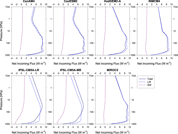
Figure 3. Vertical profiles of global-mean change in the net downward radiative flux in response to a quadrupling of CO2 computed from the double call method. Solid lines in dark blue represent the sum of longwave (dashed lines in blue) and shortwave (dashed lines in purple) components.
Download figure:
Standard image High-resolution imageThe shortwave component shows generally similar patterns of vertical distribution among the models. Minima and maxima are located at the surface and at the TOA, respectively. The difference between maximum and minimum values is less than 1 W m−2 except for the IPSL models (∼3 W m−2). At the TOA, the shortwave forcing ranges from ∼0 to greater than 1 W m−2.
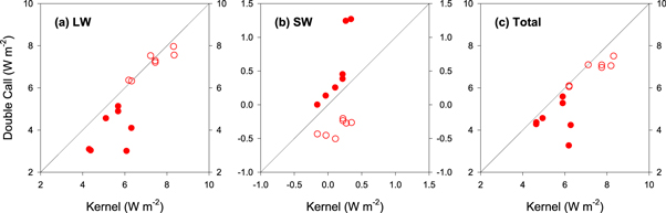
To further examine the kernel and double-call results, figure 4 compares global-mean instantaneous forcing estimated using radiative kernels with global-mean instantaneous forcing computed from the double-call method. Both of the methods indicate that the direct radiative impact of a quadrupling of CO2 shows an intermodel spread of ∼2 W m−2 for the longwave component. However substantial disagreement between the two methods exists for some models, such as HadGEM2-A and MIROC5 for which the kernel-estimated forcing is nearly twice as large as the double-call calculation. In the case of the shortwave component, most of the models have a very small instantaneous forcing and the estimates agree well for both of the methods. However the two IPSL models exhibit distinctly larger shortwave forcings from the double-call method (∼1.2–1.3 W m−2) compared to the radiative kernel method (∼0.3 W m−2). These two models have exceptionally large double-call computed shortwave forcing, given that their longwave counterpart is ∼3 W m−2. A comparison of the stratosphere adjusted forcing (i.e., the sum of instantaneous forcing and stratospheric adjustment) from the kernel method to the stratosphere-adjusted forcing from the double-calls (open circles) indicates better agreement between the two estimates, suggesting that intermodel differences in stratospheric adjustment act to compensate for part of differences in instantaneous forcing.
Figure 4. Comparison of global-mean instantaneous forcing (filled circles) for a quadrupling of CO2 between the radiative kernel method and double call method: (a) longwave, (b) shortwave, and (c) total. Open circles denote comparison of the stratosphere-adjusted forcing. Each symbol represents an individual model. Panel (b) has a smaller range. Note that the one-to-one line is shown for reference.
Download figure:
Standard image High-resolution image
The cause of the discrepancy between the double-call and kernel estimates of instantaneous forcing is not immediately clear. Because the radiative transfer model and climatological profiles used to develop the radiative kernels differ from that of the individual CMIP5 models, the kernel-method may not properly account for the contributions of the individual radiative feedbacks to the TOA fluxes. Such errors would result in erroneous estimates of the direct forcing term, since it is computed as a residual of the TOA fluxes and kernel-based calculations of radiative feedbacks and radiative adjustments. However, the adjusted forcing is also computed as the residual of the TOA fluxes and kernel estimates of the radiative feedbacks; the good agreement between the Gregory/Hansen estimates of adjusted forcing with those obtained using the radiative kernels suggests that the error in the kernel estimates is small (∼0.5 W m−2). Because the magnitude of radiative adjustments is an order of magnitude smaller than the radiative feedbacks, this implies that the uncertainties in computing the radiative adjustments from kernels are also an order of magnitude smaller (e.g. ∼0.05 W m−2). This is consistent with previous intercomparisons of radiative kernels which suggest that intermodel differences in kernel calculations are less than 10% (Soden et al 2008), although this comparison was limited to just four different kernels.
4. Summary
In this study, we compared four different methods for computing radiative forcing using climate model experiments performed for CMIP5. It is found that the adjusted forcing estimated from the alternative methods ranges from 5.5–9 W m−2 for a quadrupling of CO2 in climate models of CMIP5. Further analysis using radiative kernels and offline double-call radiative transfer calculations clearly indicates that a significant portion of the intermodel spread in adjusted forcing results from intermodel difference in the instantaneous forcing, confirming the argument of Chung and Soden (2015) that intermodel spread in the instantaneous forcing is likely related to biases in computing the radiative transfer and supports previous findings (e.g. Collins et al 2006, Forster et al 2011).
More in-depth analysis is required to attribute the causes of the intermodel spread in forcing. Potential causes that can be envisaged are uncertainty in spectroscopy or in the formulation of the radiative transfer. For instance, Iacono et al (2008) showed that correlated-k methods tend to overestimate CO2 forcing relative to line-by-line models. Since the error that results from the approximations made in broadband radiative codes in climate models hampers an in-depth analysis, a coordinated intercomparison between double-call results and line-by-line calculations such as one conducted in Collins et al (2006) could help to reduce this uncertainty. The influence of the background state on the potential differences in instantaneous forcing also warrants further attention.
Our assessment of the intermodel spread in the instantaneous forcing from CO2 is similar to that obtained by Collins et al (2006) for both the shortwave and longwave components. Collins et al (2006) documented that at the top of model the range of instantaneous forcing for a doubling of CO2 is ∼1.2 W m−2 for the longwave part of the electromagnetic spectrum and ∼0.5 W m−2 for the shortwave part. These ranges, respectively, correspond to ∼2.4 W m−2 and ∼1.0 W m−2 for a quadrupling of CO2 if the curve of growth of forcing with CO2 holds. This agreement further supports the validity of the kernel methodology. The spread is significantly larger than that obtained by Collins et al using line-by-line calculations, indicating that the spread in forcing calculations does not reflect uncertainties in radiative transfer theory, but in the fidelity of its implementation in climate models.
Given the importance of the radiative forcing in climate change projections, we suggest that radiative forcing be a routinely archived diagnostic of climate model simulations. Including offline 'double-call' radiative transfer calculations of the instantaneous forcing is essential to better documenting the cause of the intermodel differences in the projected climate response.
Acknowledgments
We would like to thank two anonymous reviewers for their constructive and valuable comments which led to an improved version of the manuscript. We acknowledge the World Climate Research Programme's Working Group on Coupled Modeling, which is responsible for CMIP, and we thank the climate modeling groups (listed in table S1 of this study) for producing and making available their model output. For CMIP the US Department of Energy's Program for Climate Model Diagnosis and Intercomparison provides coordinating support and led development of software infrastructure in partnership with the Global Organization for Earth System Science Portals. Model output analyzed in this study is available from the Earth System Grid Federation (http://cmip-pcmdi.llnl.gov/cmip5/). This research was supported by a grant from the NASA ROSES program and the NOAA Climate Program Office.