


Abstract
Understanding the changing nature of the intraseasonal oscillatory (ISO) modes of Indian summer monsoon manifested by active and break phase, and their association with extreme rainfall events are necessary for probabilistic estimation of flood-related risks in a warming climate. Here, using ground-based observed rainfall, we define an index to measure the strength of monsoon ISOs and show that the relative strength of the northward-propagating low-frequency ISO (20–60 days) modes have had a significant decreasing trend during the past six decades, possibly attributed to the weakening of large-scale circulation in the region during monsoon season. This reduction is compensated by a gain in synoptic-scale (3–9 days) variability. The decrease in low-frequency ISO variability is associated with a significant decreasing trend in the percentage of extreme events during the active phase of the monsoon. However, this decrease is balanced by significant increasing trends in the percentage of extreme events in the break and transition phases. We also find a significant rise in the occurrence of extremes during early and late monsoon months, mainly over eastern coastal regions. Our study highlights the redistribution of rainfall intensity among periodic (low-frequency) and non-periodic (extreme) modes in a changing climate scenario.
Export citation and abstract BibTeX RIS

Content from this work may be used under the terms of the Creative Commons Attribution 3.0 licence. Any further distribution of this work must maintain attribution to the author(s) and the title of the work, journal citation and DOI.
1. Introduction
A strong intraseasonal variability (ISV) discerned during the monsoon season can be envisaged as active (wet) and break (dry) episodes of enhanced and decreased precipitation over India [1–8]. Despite increasing sea surface temperature (SST) over the Indo-Pacific warm pool and global monsoon precipitation amplification [9], mean Indian summer monsoon rainfall (ISMR) has not shown any long-term trend [10–13]. Also, no such significant trends in either the days of active or break events were found [7]. It was shown that interannual variation of the Indian monsoon cannot be considered as primarily arising from the interannual variation of ISV [7], which indicates that the nature of ISV during the years of major droughts and major floods is not different [6]. On the other hand, it is found using outgoing longwave radiation (OLR) data that intraseasonal oscillation (ISO) activity is inversely related to Indian monsoon strength [4]. Although it is clear that the ISV can have an impact on the seasonal total rainfall, we still lack proper understanding of the extent of the contribution of the ISV to the interannual variation [4, 7]. However, in a global warming scenario, a very important question could be: Is there any change in intensity of monsoon ISV in the recent decades? ISOs are recognized as the building blocks of monsoon ISV, and its intrinsic chaotic character raises an important question about the predictability of seasonal mean ISMR [3, 14]. Using a number of atmospheric general circulation models (AGCMs), it was shown that higher ISV can lead to poorer predictability of seasonal mean [15]. Hence, it is important to identify any significant changes in monsoon ISO strength.
A weakening of the 30–60 days ISO in lower-tropospheric zonal wind over the Indian subcontinent, the northern Arabian Sea and the Bay of Bengal in recent decades has been observed [16]. This weakening is a response of increased SST over the Indian Ocean, which resulted in a decreased land-sea heat contrast and weaker low-level westerlies over the northern Indian Ocean and the Indian subcontinent. No change in 10–20-days ISO was observed in the Indian subcontinent region. However, given its direct socio-economic impact, rainfall can be recognized as the most important facet of the monsoon. Also, since ISV of wind and precipitation may differ, changes in the intensity of rainfall ISV using a rain-gauge dataset would give a new dimension in this direction.
Although no statistically significant spatially uniform trends were observed in maximum rainfall, increasing spatial variability of rainfall extremes exists over India [12]. Further, an increasing trend of extreme events and intense active spells in central India are observed, possibly because of more moisture content in the atmosphere [11, 17]. Extreme events can be caused by small-scale convective instabilities in the presence of moisture, or can be associated with severe cyclonic storms or synoptic-scale systems. It was suggested that increased variability in the synoptic scale, caused by a rising trend in relatively weak low pressure systems (LPS), leads to an increase in extreme events [18]. LPS are, in turn, modulated by ISOs with a proclivity to occur in active phases [19]. Given the severe societal impact of rainfall extremes [3, 5], effective flood forecasting requires rigorous investigation of the relationship between ISO modes and extreme events, especially in the current scenario where extreme rainfall events are increasing globally [20].
In spite of outstanding advancements in numerical modeling and computation in recent decades, a high degree of uncertainty in medium- or long-range prediction of such extreme events still persists. This uncertainty can be lessened by proper assessment of extreme rainfall characteristics and its relationship with periodic modes. Adaptation and mitigation of climate changes related to intraseasonal variability can be harder compared to the changes in time-mean rainfall, necessitating a better understanding of the relationship between ISOs and extreme events, better forecasts on a subseasonal-scale, and effective risk management of extreme events. Here we examine whether the intensity of monsoon ISO modes is changing, and with the increasing overall number of extreme events, how they were associated with the phases of ISOs in the past few decades.
2. Dataset
We used daily gridded rainfall data (1° x 1°) over India for 1951–2013 from the India Meteorological Department (IMD) [21]. This dataset is based on quality controlled daily rainfall measured at 2140 stations, well distributed over India, and has been extensively used to understand monsoon behaviour [11, 12, 17, 21, 22]. Extreme northern part of India and a few gridpoints over the northeast regions are not considered in the study.
3. Extracting ISO modes and defining active/break phases
3.1. Low and high-frequency ISOs
Since our interest lies in the intraseasonal scale, we initially filter out any temporal scale beyond the intraseasonal period (8–90 days) from 63 years (1951–2013) of data at each gridpoint using a Fourier filter to obtain a more coherent analysis. We capture the ISO modes by applying multichannel singular spectrum analysis (MSSA) to the May–October (184 days long) data over India for each year [23]. This separates out oscillatory modes from noisy data, following which we determine the spatial-temporal structures associated with those characterized by that part of the spectrum. (A brief detail of MSSA with the parameters used here can be found in supplementary information, SI README available at stacks.iop.org/erl/10/054018/mmedia.)
The eigenvalues obtained from MSSA represent the power in the extracted modes. When we apply MSSA to rainfall data, several oscillatory modes, occurring usually in pairs, are detected every year, and are significantly different from those generated by pure noise. These significant oscillatory modes have periodicities within the 10–60-day window, and together they exhibit the nature of a broad spectrum in monsoon ISOs. Different significant oscillatory pairs show distinct spatio-temporal characteristics with varying intensity each year, but in general, 20–60-days periodic oscillations show northeastward propagation, replicating the typical active-break cycle [6], and 10–20-day oscillations propagate northwestward [1]. Using the year 1951 as an example, eigenmodes 1 and 2 with periodicities of the 37-day and eigenmodes 4 and 6 with periodicities of 14 days stand out as significant modes (figure S1). The 37-days periodic pair (RC(1,2)) shows a northeastward movement with phase 1 in the phase-composite structures showing a developing stage of an active period with positive rainfall anomalies over southern peninsular India. This positive rainfall anomaly propagates northward and gets established in central India in phases 4 and 5. In phases 7 and 8 the positive anomaly weakens and moves towards the foothills of the Himalayas. A similar structure can be found for break periods, and phases 1–4 are seen to be almost opposite of phases 5–8. The 14-day periodic pair (RC(4,6)) also shows propagation but in the northwestward direction from the eastern coast of India to the northwestern part. However, the amplitude of RC(4,6) is slightly less than RC(1,2). A few more oscillatory modes come up as significant for 1951, but more or less, the spatio-temporal characteristics of those modes can be classified as northeastward propagating (20–60 days periodic) or north-westward propagating (10–20 days periodic).
For simplicity, hence, we divide the significant oscillatory modes for each year into two scales: low (20–60 days) and high frequency (10–20 days). Reconstruction of the intraseasonal features in each scale is done by extracting all the significant eigenmodes in their respective frequency scales. This ensures that the propagation characteristics of a scale are represented by all the significant oscillatory modes. We call these reconstructed parts associated with each low- and high-frequency intraseasonal scale low-frequency ISO (LF-ISO) and high-frequency ISO (HF-ISO), respectively. The sums of the variances explained by the significant eigenmodes in low- and high-frequency scales represent the intensities of LF-ISO and HF-ISO each year relative to the total power in the intraseasonal band, and we define the respective sums as the LF-ISO and HF-ISO indices.
3.2. Active/break phases of ISO
Based on the oscillatory behaviour of the reconstructed ISOs, we defined the active (positive), break (negative) and transition phases using the ISO time series (LF-ISO or HF-ISO) and their derivatives for each year at every gridpoint (SI README and figure S2). This classification, therefore, purely depends upon the nature of the eigenmodes determined by MSSA. We determine the phases of LF-ISO and HF-ISO separately. Typically, there are 4–6 LF-ISO cycles in one May–October season.
4. Defining extreme rainfall events
A large spatial variability in climatological mean and variance of May–October daily mean rainfall can be seen over India (figure S3). The Western Ghats and northeastern India receive most of the rainfall with large variability. Over the central Indian region, mean and variance are quite homogeneous. However, an important aspect is that the spatial distribution of mean and variance are highly correlated (corr. coeff. = 0.90). The spatial inhomogeneity in mean and daily variability of monsoon rainfall prevents us from defining a fixed threshold for an extreme event across the entire country. We set the 99.5th percentile value (results are insensitive to small changes in percentile threshold) at each gridpoint based on May–October data for 1951–2013 to define the threshold of an extreme event. So, each location has a different threshold for extreme rainfall, e.g., over central India it is almost 90–100 mm/day, and over 130 mm/day in the Western Ghats (figure S3). This threshold more or less agrees with the threshold for extreme events defined in [11].
5. Results
5.1. Weakening of low-frequency ISO
The time series of the LF-ISO and HF-ISO indices are shown in figures 1(a) and (b). The indices show large variability during 1951–2013, and we find a significant decreasing trend (2% significance level) in the LF-ISO intensity with HF-ISO variance remaining almost constant for the entire time period. The negative correlation (corr. coeff. = −0.52) between LF-ISO and HF-ISO intensities indicates their compensating behaviour to each other. A point to note is that here we calculate the percentage of the variance explained by the LF-ISO and HF-ISO to the total 8–90-day band (which may contain noise) variance in May–October each year. This implies that although the variance of the area-averaged summer monsoon rainfall over central India is significantly increasing [11], the relative contribution from LF-ISO is decreasing.
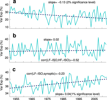
Figure 1. Time series of the cumulative variance explained by the significant eigenmodes (in percentage of the intraseasonal band (8–90 days)) that represents oscillatory behaviour with periodicities of (a) 20–60 days and (b) 10–20 days. (c) Time series of the calculated percentage of the total daily variance explained by 3–9-day filtered rainfall averaged over India every year. Trends are evaluated using a Theil-Sen estimator, and the Mann-Kendall test is used to determine the significance of the trends (see SI README available at stacks.iop.org/erl/10/054018/mmedia).
Download figure:
Standard image High-resolution imageThis loss in LF-ISO intensity is balanced by a significant increasing trend (1% significance level) in synoptic-scale (3–9 days filtered) variability (figure 1(c)). The increase in synoptic-scale variability is already documented over central India [18] with a rising trend in the frequency of weak LPS in recent decades [18, 24]. Notably, although there is a decrease in more intense systems, an increasing trend in weak LPS outweighs this reduction [18, 24] and is associated with the increase in synoptic variability.
Amplitude and distribution of LF-ISO related rainfall strongly vary from year to year [4, 25]. For example, the 1973 summer is marked by four distinct northward propagating active cycles and are separated by almost 40 days (figure S4). This vigorous ISO activity is captured in figure 1, where we get maximum LF-ISO intensity in 1973, whereas in 1984, LF-ISO activity is virtually absent (figure 1 and figure S4). A clear understanding of the causes behind these interannual changes in ISO intensity is not yet achieved, but is required for better prediction [15]. However, [26] has experimentally shown that the northward propagation of convection is more regular with slower frequency during warm ENSO (El Niño and Southern Oscillation) periods.
Most of the variability of LF-ISO is seen over the western coast and central India (figure 2(a)), because the LF-ISOs propagate in the northeastward direction from the equatorial Indian Ocean through these regions (figure S1). Favourable conditions for the formation of lows in the Bay of Bengal cause more synoptic variability over the eastern coast (figure 2(c)). However, in the post-1980 period, the LF-ISO variability decreased over west and central India, and parts of peninsular India, with an increase in synoptic variability (figures 2(d) and (f)). (To understand the changes in spatial pattern of the trends we saw, we divided the entire time series into two epochs: pre-1980 (1951–1980) and post-1980 (1981–2010).) This perhaps indicates a decline in the number of long-duration rain events with an increase in short rain episodes and dry spells in the region [22]. HF-ISO variability is mostly seen over the monsoon trough and remained almost the same after 1980 (figures 2(b) and (e)).
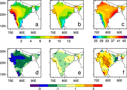
Figure 2. Spatial distribution of the percentage of the total daily variance explained by the (a) LF-ISO, (b) HF-ISO and (c) 3–9-day filtered rainfall, respectively, during May–October for 1951–1980. (d)–(f) Post-1980 minus pre-1980 for the same scales showing the spatial change in variability in these two time periods. Stippling indicates regions where the null hypothesis of equal means in pre-1980 and post-1980 period can be rejected at 10% significance level.
Download figure:
Standard image High-resolution imageIt is intriguing to know the factors that may have played a role in weakening the intensity of LF-ISO. It has been shown that rising SST over the Indian Ocean could be a factor in weakening the 30-60-day ISO in zonal wind over the Indian region [16]. Recent studies indicate upper tropospheric (200hPa) warming over the equatorial Indian Ocean related to enhanced deep moist convection due to warmer SST, and cooling over the Tibetan plateau produces a significant decreasing trend of the meridional temperature gradient over the monsoon region at that level [27]. This, in turn, weakens the tropical easterly jet via the thermal wind balance and causes a significant decrease in the prevailing easterly vertical shear during the monsoon season (figure S5). Easterly shear essentially catalyses the coupling between free-atmosphere baroclinic and barotropic modes and generates barotropic vorticity to the north of a convective zone. This shifts the moisture convergence in the boundary layer towards the north, and thus the northward propagation of convection occurs [28]. Therefore, weakening of easterly shear can be one possibility towards the debilitation of the intensity of the northward-propagating LF-ISO modes. However, it was also deduced in [28] that the phase speed of the most unstable mode (ISO) is linearly proportional to the vertical shear intensity. But we did not see any change in the mean LF-ISO periodicity in our analyses. Also, the simultaneous correlation between vertical shear or meridional temperature gradient and LF-ISO intensity is not significantly high, indicating the involvement of other important factors in controlling the LF-ISO intensity. On the other hand, northward-propagating ISOs in the Indian subcontinent are shown to be associated with the eastward movement of convection near the equator [29]. This indicates that the dynamic parameters influencing the equatorial ISOs also need to be studied carefully to understand the observed trends.
5.2. Association with extreme events
In order to understand how the occurrence of extreme events is associated with LF-ISO, we looked into the phase composite structures of LF-ISO and the number of extreme events occurring in a particular phase composite. We find that extreme events are inclined to occur in places where LF-ISO is positive (this can be referred to as the active phase of LF-ISO) and consequently, they propagate northeastward in tandem (figure S6). The maximum number of extremes occurs when the active phase of LF-ISO is over central India. However, this association is not prominent for the HF-ISO case (figure not shown). This essentially states that extreme rain events are preferentially located in the monsoon lows or large-scale convergence zone and propagate poleward as the LF-ISO progresses. When the LF-ISO reaches the central Indian region, it becomes most intense, and the maximum number of extreme events occurs during that phase compared to the other phases (phase 3 in figure S6). An important point to make here is that we do not assume that extreme events are caused by the LF-ISO. Our understanding to date is not sufficient enough to conclude that any particular extreme event is solely because of LF-ISO, HF-ISO, synoptic-scale disturbance or boundary forcing such as ENSO-related activities. Hence, the discussion is not based on the attribution of extreme events to LF-ISO; it is just an association of events that take place.
Against the backdrop of decreasing intensity of LF-ISO, this association of LF-ISO and extreme events can be crucial for the better prediction of the climatic extremes. To address this issue, we looked into the distribution of occurrences of extreme events in the active, break and transition phases each year. Evidently, extreme events are most frequent in the active phase of LF-ISO, with the fewest occurring in the break phase (figure 3). There is a significant increasing trend (1% significance level) in the number of extreme events (figure 3(a)), which is in tune with previous studies [11, 17]. Nevertheless, there is a significant decreasing trend in the percentage of extreme events occurring in the active phase compared to the total number of extreme events over India (5% significance level) (figure 3(d)). This decrease is offset by significant increasing trends in the percentage of extreme events during the break and transition phases compared to the total number of extreme events (10 and 5% significance level, respectively) (figures 3(b) and (c)). Both active-to-break and break-to-active transition phases show significant increasing trends (figure not shown). This suggests that in the recent decades, the association between LF-ISO and extreme events is changing, and there exists a propensity for more extreme events to occur during the break and transition phases in recent decades than in the earlier decades. Note that the actual numbers of extreme events that occur in different phases of LF-ISO over India are significantly increasing, but the percentage of extreme events occurring in the active phase of LF-ISO each season shows a negative trend.

Figure 3. (a) Yearly occurrence (N) of extreme events over India during May–October, 1951–2013. Time series of the percentage ratio of the extreme events that occurred in the (b) negative (break) phase, (c) transition phase and (d) positive (active) phase of LF-ISO, respectively, to the total number of extreme rainfall events each year over India. Trends and significance levels of the trends are calculated as in figure 1. Spatial distribution of the percentage of the extreme events occurred in May–October during 1951–1980 in the (e) negative (break) phase, (f) transition phase and (g) positive (active) phases of LF-ISO, respectively. (h)–(j) Post-1980 minus pre-1980 for the same showing the spatial pattern of difference in extreme events occurring in these two periods in different phases of LF-ISO. Stippling indicates regions where the null hypothesis of equal means in the pre-1980 and post-1980 periods can be rejected at 10% significance level.
Download figure:
Standard image High-resolution imageOver the central Indian region, extreme events show a greater tendency to occur during the active phase of LF-ISO. However, over northeast and peninsular India, a large number of extreme events (almost 40%) occur during the transition and break phases (figures 3(e)–(g)). Interestingly, the percentage of extreme events occurring in the break and transition phases shows an increase over the Gangetic-Plain, eastern coast and southern part of India during the post-1980 period. Consequently, the percentage of extreme events in the active phase in these regions has decreased (figures 3(h)–(j)). A possible cause could be the warming trend in SST that could create a conducive environment for the formation of LPS [18, 24]. But changes in the monsoon trough warrant further investigation, as extreme events here are generally embedded in large-scale ISV, and perhaps can be best answered using regional modeling studies. Essentially, the weakening intensity of LF-ISO and the redistribution of extreme events in different phases of LF-ISO show the gravest impact over the most productive agricultural regions in India (i.e., central India and the Gangetic Plain), where irrigation is largely dependent on monsoon rainfall. (Stippled regions are hardly present in (h) because of very few non-zero values in either of the epochs at each gridpoint. The results are, in this case and also in (i) and (j), suggestive but not conclusive, and a larger dataset may be needed to bring out this difference more significantly.)
5.3. Early- versus late-monsoon extreme events
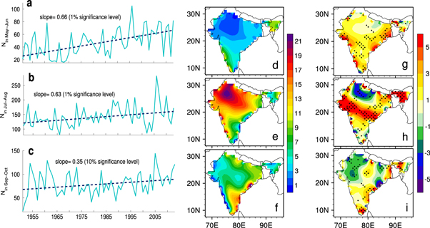
We also find that there is a significant rise (1% significance level) in the number of extreme events during early monsoon (May–June) and peak monsoon (July–August) seasons with an almost 3-fold increase in May–June (figures 4(a)–(b)). An increase in extreme events during late monsoon months (September–October) also occurs, but the slope is comparatively smaller (figure 4(c)). Extreme events over central India occur most frequently during July–August with fewer events in May–June (figures 4(d)–(f)). Over peninsular India and the eastern coastal region, extreme events are more common during the late monsoon months. There is a 5-fold increase in extreme events over the coastal regions during May–June in the post-1980 period with a rise almost all over India (figure 4(g)). Extreme events in July–August have increased over all of India, except the northern region, in the post-1980 period with almost a 2-fold increase over northeastern India (figure 4(h)). During late monsoon months, the number of extreme events increased over the peninsular and northeastern part with a decrease over a few regions in the northwest and east of India during post-1980 period (figure 4(i)). (Because of very few non-zero values in either of the epochs at each gridpoint, the results (figures 4(g)–(i)) are suggestive but not conclusive, and a larger dataset may be needed to bring out this difference more significantly.)
Figure 4. Extreme events occurred during 1951–2013 in (a) May–June, (b) July–August and (c) September-October over India. Trends and significance of these trends are calculated as in figure 1. Spatial distribution of the total number of extreme events occurred in 1951–1980 for (d) May–June, (e) July–August and (f) September–October over India. (g)–(i) Difference for the same between the 1981–2010 and 1951–1980 epochs. Stippling indicates regions where the null hypothesis of equal means in the pre-1980 and post-1980 periods can be rejected at 10% significance level.
Download figure:
Standard image High-resolution image
We also examined the changes in the occurrence of extreme events during different LF-ISO phases in the previously mentioned 2-month periods. A steeper rise in the total number of extreme events in May–June over India is found in break and transition phases compared to the active phase (figure not shown). However, extreme events in September–October are nearly stable in all three phases over all of India. During these two months, extreme events in the break and transition phases tend to occur mostly over the eastern coast and peninsular India. A significant increase in the extreme events in the break phase is found in the post-1980 period over these regions. This indicates that in the late monsoon period, extreme events are now more likely to occur in the break and transition phases over the eastern coastal and peninsular regions. The active phase spatial patterns for extreme events are more or less similar to figures 4(d)–(i), as active phase extreme events contribute to almost 80% of the total extreme events for all the 2-month periods.
6. Conclusions and discussion
Using MSSA we extracted and examined the strength of ISO modes in Indian monsoon rainfall and found a significant decreasing trend in the relative strength of low-frequency ISO. In addition, the synoptic variability over the Indian region has increased significantly, mainly over central India. Using a percentile-based threshold for extreme rainfall, we also found the relative number of extreme events during the active phase of LF-ISO has decreased significantly in recent decades with significant increases in the break and transition phases, counterparts, thus indicating a redistribution of the preferred time of extreme events within an intraseasonal timescale. Essentially, although the number of extreme events has increased remarkably over the past six decades, the ratio of extreme events occurring in the active phase of LF-ISO compared to the total number of extreme events in a particular season has decreased significantly. We performed similar analyses of extreme events with the HF-ISO, but observed no significant trends. We checked the robustness of our results by performing MSSA with non-Fourier filtered data and found that the trends and spatial patterns are qualitatively similar. We also found that there is a sharp increase in the number of extreme events during the early monsoon period (May–June), mainly over the coastal regions, along with a significant increase in extreme events over most of India, except a few regions in the northern part during the peak monsoon time (July–August). Moreover, during late monsoon months (September–October) the number of extreme events increased over the eastern coast, particularly during the break and transition phases of LF-ISO.
Therefore, increased rainfall during the break/transition phases (in the form of extreme events) in the recent decades could be a contributing factor to a reduction in LF-ISO intensity through changes in its amplitude and variability. But the causality of such a phenomenon warrants rigorous investigation. These sporadic extreme rainfall events diminish the low-frequency variability, which can impact the potential predictability of wet and dry spells. More importantly, the fitful occurrence of these short spatial and temporal-scale extreme events would make it more difficult to capture in medium- and long-range forecasts.
It is worth noting that the variability of LF-ISO intensity has increased since mid-1970s (figure 1(a)), which can be considered as a part of the multi-decadal shifts. However, multi-decadal shifts can be hard to detect using 63 years of data. In spite of this constraint, we checked the changes in the spatial pattern of ISO variability using different segments of time series and they are consistent with our results. A slight increase in LF-ISO variability was found over central India during the 1995–2013 period compared to the 1980–1995 period, but a multi-decadal variability requires more evidence. Hence, without denying the possibility of a multi-decadal shift, we report here a decreasing trend in LF-ISO intensity. Identifying multi-decadal shifts (no such discernible shifts are shown in figure S5) and finding the exact dynamic reasons for it can be challenging since the intensity change in LF-ISO over India during monsoon season can be attributed to various factors, such as its relationships with the Eurasian continent, Pacific decadal oscillation (PDO), ENSO, the Indian and Atlantic Ocean SSTs, and even aerosols. Each of these factors warrants careful research prior to concluding what factors may have played a role in controlling the interannual variability of low-frequency ISV intensity.
It has been shown in various studies that the monsoon circulation over the Indian region has weakened because of reduced land-sea thermal contrast in recent decades [16], which may be attributed to spatially uneven effects of greenhouse gases [30] or human-influenced aerosol emissions [13, 31]. But there is no consensus as yet on how the ISO modes will behave in a changing climate, and it remains a very difficult problem to be addressed, as the state-of-the-art models still have difficulties in simulating the mean picture of ISO. Based on the observational dataset, our results can constitute a concrete step toward unravelling the hydrological impact of climate change on the intraseasonal scale. However, further investigation is required to comprehend the dynamic reasoning (both internal dynamics and boundary forcings) behind the observed changes with a better understanding of the interaction between different ocean and atmospheric variables at different scales [13, 20]. A proper assessment of local- and regional-scale land-use change is also required to understand the observed changes.
Acknowledgments
The high-resolution gridded daily rainfall data we use here have been developed by the India Meteorological Department (IMD) for the period 1951 to 2013 [21]. The dataset can be obtained by contacting the National Climate Centre, IMD, Pune (ncc@imdpune.gov.in). We thank MoES/CTCZ and DST, Government of India, for funding this research, and Prof N V Joshi (CES, IISc) for helpful discussions. The comments from two anonymous reviewers are greatly appreciated.