

Abstract
The evaluation of precipitation extremes is a paramount challenging issue in climate sciences and there is a need of both assessing changes in climate projections and comparing climate model simulations with observations. To address these needs, a non-parametric approach specifically designed for extremes is here proposed. The method is tested and applied to observations and CMIP5 historical simulations and future projections (under the high emission scenario RCP8.5) over the Euro-Mediterranean region. Results support the existence of a scaling relationship among models and between models and observations in terms of conditional mean of the extremes. However, the rescaled tails of models' precipitation show significant differences when compared with observations. Concerning future projections, models show an intensification of heavy precipitation (especially at the end of the 21st century) linked to a change in the conditional mean of extremes. More complex changes in the upper tails are not identified at the mid-century, while a lack of model agreement prevents drawing definitive conclusions for the end of the century.
Export citation and abstract BibTeX RIS

Content from this work may be used under the terms of the Creative Commons Attribution 3.0 licence. Any further distribution of this work must maintain attribution to the author(s) and the title of the work, journal citation and DOI.
1. Introduction
Precipitation extremes represent a global threat, especially in a climate change context where both their frequency and intensity are expected to change (IPCC 2012). Since exposure and vulnerability to climate extremes are both dynamic and determined by several socio-economic and political factors (IPCC 2012), also the impact of precipitation extremes can significantly change. Recent studies (Kharin et al 2013, Toreti et al 2013) have investigated the behavior of those extremes in the next decades of the 21st century by analyzing global climate models (GCMs) projections. These studies have shown an intensification of return levels (e.g., 20, 25 and 50 years) almost everywhere in the world, but with reliable and consistent results restricted to specific seasonal-dependent areas over the mid-high latitudes of both hemispheres (Toreti et al 2013). Those findings, the large uncertainty still characterizing the estimation of precipitation extremes (Hofstra et al 2009, Trenberth 2011) as well as the identified model issues (Min et al 2011, Sperber et al 2013), point at the need of a better evaluation of climate model simulations as well as of their projected changes. Concerning the comparison of historical simulations with the available observations, several issues arise when the focus is on extreme precipitation (Randall et al 2007). Previous studies have usually applied Taylor diagrams (Taylor 2001) to return levels (Toreti et al 2013, Wehner 2013); however, this approach does not allow directly comparing observed and simulated tails. Weller et al (2013) proposed and applied an approach based on tail-dependence, while other studies (Chan et al 2014) have compared the estimated parameters of imposed extreme value distributions. As for the assessment of the significance of the projected changes, recent studies have usually focused on the comparison of projected return levels with the return levels estimated for the historical simulation by looking at the obtained confidence intervals (Goubanova and Li 2007) or by applying some classical statistical tests not specifically developed for tail-comparison (Kharin et al 2013). Finally, only few studies have dealt with the inter-model comparison in terms of tails of the distributions (Weller et al 2013, Chan et al 2014).
Here, we propose a statistical approach that can be applied to address the aforementioned issues. The following section gives the details of the method. Section 3 deals with the analysis of eight global climate model runs done in the framework of the Coupled Model Intercomparison Project Phase 5-CMIP5 (Taylor et al 2012). Finally, the last section focuses on the main conclusions and the discussion of some key issues.
2. The method
Several statistical tests exist for the comparison of two samples thought as realizations of two different (under the alternative hypothesis) distributions, for instance: Kolmogorov–Smirnov and Cramer von Mises (Shao 2003). Those procedures mainly focus on the central part of the distributions rather than on the tails. Therefore, if the interest is on extremes (i.e., high values above a certain threshold far from the central part of the distribution) another approach giving more weight to the tails is needed. In a parametric framework, Heo et al (2013) and references therein evaluated the performance of several different tests against a modified Anderson–Darling test (Ahmad et al 1988) by imposing extreme value distributions. Here, we propose a flexible and not dependent on some extreme value theory (EVT) assumptions (e.g., being in the domain of attraction of an extreme value distribution) non-parametric two-sample testing procedure. The proposed method has been inspired by the work of Pettitt (1976) and it is based on a two-sample modified Anderson–Darling statistic. Let  and
and  be two continuous random samples. The modified two-sample Anderson–Darling statistic is:
where  and
and  are the survival empirical distribution function of X and Y, respectively, and
  represents their weighted average. The proposed procedure is based on
  (see the appendix and the supplementary material for further details, available at stacks.iop.org/erl/10/014012/mmedia). The null hypothesis of equal distributions can be rejected when T is greater than the approximated critical value at the chosen significance level (here 95%). The method can be applied either to the entire set of X- and Y- values (e.g., all rainy days) or (when the interest is only on extreme events) to the rescaled tails, that is, all the excesses above high thresholds u and v (here, the 90th percentiles) conditional on
  and
and  :
:  and
and  . Here,
  and
and  represent, respectively, the conditional mean of Xe and Ye:
  and
and  . The use of rescaled tails enables to isolate the effect of simpler changes in the conditional means and to focus on more complex (and potentially increasing the risk associated with extremes) changes in the tail behavior (e.g., longer tails). To analyze the CMIP5 model simulations, the latter approach was followed. Since each grid point was tested separately, the significant values were identified by using the approach of Genovese and Wasserman (2004) to address the type I error issue of multiple testing (see the supplementary material for details). Additionally, since the proposed procedure only estimates the absolute difference of two distributions, the sign (i.e., the direction of change) is assessed by using the Kullback–Leibler direct divergence (hereafter, KLD-divergence):
where fe and ge are the densities of  and
and  , respectively. This divergence can be non-parametrically estimated as proposed by Naveau et al (2013) and more details are given in the supplementary material.
To better evaluate the proposed procedure, all rescaled excesses were also analyzed by using the approach proposed by Naveau et al (2013) fully based on divergence (see the supplementary material).
3. Results
3.1. Method assessment on simulated data
To assess the behavior of the proposed procedure in critical conditions with two not too different tails (e.g., exponential versus heavy tailed), simulations similar to the ones of Naveau et al (2013) were carried out. Extreme value distributions represent the natural theoretical environment for the statistical analysis of extremes in the so called EVT (de Haan and Ferreira 2006). Since in EVT, excesses over a high threshold can be modelled by using the generalized Pareto (hereafter, GP) family (Coles 2001), samples were generated according to GP distributions which are characterized by two parameters: σ and ξ. The latter identifies the three different tails, i.e., bounded ( ), exponential (
 ) and heavy-tailed (
 ). Several tests, with sample sizes from 100 to 10000, constant σ and different values of ξ, were performed. As shown by table S1 in the supplementary material, if the sample size is small and the shape parameters of the two samples are close, the method tends to accept the null hypothesis of equal distribution. This highlights an intrinsic feature in discriminating between different tails. If one of the distributions (of the two samples) is heavy tailed a large sample is needed.
3.2. CMIP5 model analysis
The proposed method was applied to winter (December to February) and autumn (September to November) daily precipitation data over the Euro-Mediterranean region generated by eight high resolution (spatial resolution higher than 1.5°) CMIP5-GCMs (table S2). Model runs were remapped on a common  grid by using a conservative remapping scheme (Chen and Knutson 2008, Jones 1999). Historical simulations (1966–2005) and two future time periods (2020–2059 and 2060–2099) under the high emission scenario RCP8.5 (Taylor et al 2012) were analyzed as well as the gridded daily observations of the E-OBS dataset (Haylock et al 2008). Complementary to the test, the existence of a simple linear relationship between the tail scaling factors (i.e, the conditional means of the excesses of the models
  and of the observations
  ) was investigated by applying a Spearman-based spatial correlation analysis in the period 1966–2005. Then, also the ratio of the estimated models' scaling factors for the two future time periods w.r.t. the historical period was computed,
  , to identify changes in the climate projections. The inter-model comparison and the comparison of each model with the gridded observations in the historical period (1966–2005) reveal interesting features (figures 1, 2, S1 and S2). In winter, a simple linear relationship seems to hold between the scaling factors of all models, but it is much weaker when simulations and observations are compared (figure 1). However, as shown in figure 1, better results are achieved if the southern part of the domain is not included in the assessment. This effect might be caused by some data issues affecting E-OBS in areas where not so many stations are available. Similar results can be observed in autumn (figure S1). A further look to the model-observation comparison (figures 2 and S2) shows that remarkable spatial differences as well as similarities among models exist for the rescaled tails. In winter, tails in the southern part of the domain are over-simulated by all models, while the rest of the domain shows under-simulated tails, with some local exceptions such as in southern Spain and France (figure 2). The same holds for autumn (figure S2). Similar findings can be observed by replacing the Anderson–Darling method with the divergence method of Naveau et al (2013) (not shown).
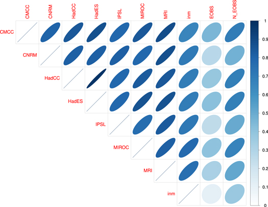
Figure 1. Spearman-based spatial correlation matrix of the tail scaling factors, estimated for the eight GCMs,  , and the gridded observations E-OBS,
  , in the winter period 1966–2005. The colors and the shape of the ellipses are associated with the correlation values. The last column refers to the same analysis without the southern part of the domain (South of 38.25° North).
Download figure:
Standard image High-resolution image
Figure 2. Rescaled-tail comparison of model simulations during the historical winter period and E-OBS. Colors are associated with the values of the two-sample modified Anderson–Darling statistic with the sign given by the estimated KLD-divergence. Blank areas are associated with non-significant values.
Download figure:
Standard image High-resolution imageConcerning the projections for the 21st century, figure 3 highlights that in winter and for both future periods (2020–2059 and 2060–2099), a slight increase (w.r.t. the period 1966–2005 and higher at the end of the current century) characterizes the conditional mean of the excesses (i.e., the estimated tail scaling factors), except for the inm model. As shown in figure 3, large spatial variability affects the majority of the models (e.g., HadES). Similar findings can be observed in autumn (figure S3). The projections for the mid-century (figures 4 and S4) do not show a significant signal in the rescaled tails, expect over north-western Africa mainly in the CMCC run (and the HadES run in winter) and some local significant changes in the other models (e.g., IPSL). The divergence method of Naveau et al (2013) provides similar findings (not shown). At the end of the century (2060–2099), a significant signal emerges in some models (figures 5 and S5), however with a lack of model agreement. In winter, longer/heavier tails are estimated over the central-eastern part of the region for the CMCC run, more restricted to the North for the IPSL simulation and to some specific areas for the MIROC, HadES and HadCC simulations (figure 5). While, almost no significant changes are estimated for three models out of eight. The African part of the domain seems to be affected by a significant tail-reduction, but with remarkable inter-model differences. Concerning autumn, similar results can be observed in figure S5, with significant changes mainly in the CMCC and IPSL runs (as in winter). The results obtained with the method of Naveau et al (2013) show similar patterns for the CMCC and IPSL runs; the other models (especially CNRM, HadES and MIROC) show more grid points affected by significant changes but a larger spatial noise (not shown).
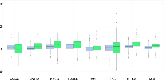
Figure 3. Boxplots of the ratio between the estimated conditional means of the excesses for the future winter time periods (2020–2059: blue; 2060–2099: green) and the historical simulations,  , derived for each grid point in the domain.
Download figure:
Standard image High-resolution image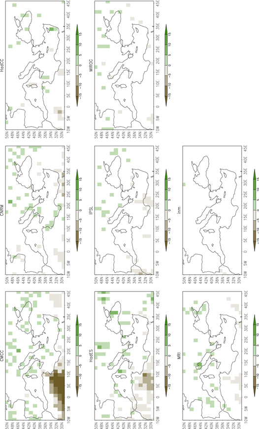
Figure 4. Results of the rescaled-tail comparison of the winter period 2020–2059 w.r.t. the historical simulation (1966–2005). Colors are associated with the values of the two-sample modified Anderson–Darling statistic with the sign given by the estimated KLD-divergence. Blank areas are associated with non-significant values.
Download figure:
Standard image High-resolution image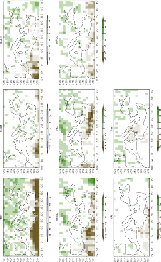
Figure 5. As figure 4, but for 2060–2099.
Download figure:
Standard image High-resolution image
4. Discussion and conclusions
Evaluating precipitation extremes is a paramount challenging issue in climate science. Here, we developed and proposed a non-parametric method to assess differences in the upper tails of distributions without imposing parametric distribution function. Statistical simulations revealed the value of the procedure as well as the classical issues (Naveau et al 2013). Good performances are achieved when large samples (having not so close associated shape parameters) are tested. This may be related to an intrinsic property of the extreme value distributions. Rare events mean small samples and consequently a higher chance to fail to reject the null hypothesis. From a practical point of view, this implies that when no significant differences in the tails are detected nothing should be concluded and high uncertainty should be assigned to those cases.
The analysis carried out on the CMIP5-GCMs over the Euro-Mediterranean region shows that a simple linear relation between the conditional mean of the excesses of models and observations seems to exist (leaving out the southern part of the domain). But the rescaled tails still have a significantly different behavior characterized by an under-estimation (over-estimation) in the northern/central (southern) part of the region. As for the projections for the mid-21st century, almost all models show an increase of heavy precipitation due to an increase in the scaling factor, but no significant changes in the tail behavior. At the end of the century, heavy precipitation continues to increase, as the scaling factors increase, but projections are not consistent w.r.t. the tail behavior. These findings seem to point at the role of the increased scaling factors in the estimated and reported (Kharin et al 2013, Toreti et al 2013) future intensification of precipitation extremes, while higher uncertainty still characterizes the tail behavior.
Acknowledgments
We thank two anonymous reviewers for their comments and suggestions that helped to improve this study. P Naveau's work has been supported by the LEFE-Multirisk and eXtremoscope projects.
: Appendix
The statistic A can be derived as follows,
where  , i.e. the number of Xʼs less equal the ith smallest value in the pooled sample. Under the null hypothesis (i.e., X and Y have the same distribution) the first two moments of A can be derived by noticing that Mi is hypergeometric distributed:
By applying by the same arguments of Pettitt (1976) and Scholtz and Stephens (1987), it can be proved that under the null hypothesis, the proposed statistic converges in distribution to the same limiting distribution of the modified Anderson–Darling statistic (Luceño 2006 and references therein). Thus, the critical values can be approximated by using the result of Sinclair et al (1990). For more details, the reader is referred to the supplementary material.