Abstract
Olfactory receptors evolved to provide animals with ecologically and behaviourally relevant information. The resulting extreme sensitivity and discrimination has proven useful to humans, who have therefore co-opted some animals' sense of smell. One aim of machine olfaction research is to replace the use of animal noses and one avenue of such research aims to incorporate olfactory receptors into artificial noses. Here, we investigate how well the olfactory receptors of the fruit fly, Drosophila melanogaster, perform in classifying volatile odourants that they would not normally encounter. We collected a large number of in vivo recordings from individual Drosophila olfactory receptor neurons in response to an ecologically relevant set of 36 chemicals related to wine ('wine set') and an ecologically irrelevant set of 35 chemicals related to chemical hazards ('industrial set'), each chemical at a single concentration. Resampled response sets were used to classify the chemicals against all others within each set, using a standard linear support vector machine classifier and a wrapper approach. Drosophila receptors appear highly capable of distinguishing chemicals that they have not evolved to process. In contrast to previous work with metal oxide sensors, Drosophila receptors achieved the best recognition accuracy if the outputs of all 20 receptor types were used.
Export citation and abstract BibTeX RIS

Content from this work may be used under the terms of the Creative Commons Attribution 3.0 licence. Any further distribution of this work must maintain attribution to the author(s) and the title of the work, journal citation and DOI.
Introduction
Animals detect volatiles in the environment with species-specific sets of olfactory receptor proteins. These olfactory systems have evolved to confer adaptive advantages in numerous different ecological niches, some of them involving chemosensory specialization, others optimized to work across a broad range of possible chemical stimuli. For a long time, humans have co-opted animal olfactory systems for their own purposes. We assume that humans first exploited the dog's sense of smell to assist in hunting, which largely involves the dog's natural behaviours. More recently, however, humans' use of animal olfaction has expanded to a wider range of species and a number of tasks that require detection or discrimination of odourants possibly unrelated to the environment in which those species have evolved (Leitch et al 2013). The question therefore arises, how effective are animal olfactory systems in parsing a set of odourants that the animal did not evolve to detect? The answer to this question is also relevant to the field of machine olfaction, because the types of chemosensors used in this field tend to be generic, rather than being heavily selected for any specific task.
Machine olfaction seeks to mimic the ability of animal olfactory systems to classify complex mixtures of volatiles into meaningful categories. Both artificial noses and biological noses contain a set of sensors (sensor types) that transduce certain features of molecules into electrical signals. In electronic noses (e-noses) transduction can be electrical, vibrational, gravimetric or optical. In biological noses, the sensors are receptor neurons containing receptor molecules that, in binding chemicals, change the membrane potential of the receptor neuron. In both cases, each sensor type is able to detect a range of different molecules, albeit with different sensitivities and, usually, there is considerable overlap between the 'receptive fields' of individual sensor (receptor) types. In e-noses, the signals from the sensors are fed into a data analysis system that can distinguish the input volatiles and classify them into meaningful categories as, presumably, occurs in an animal's brain. In contrast to methods of chemical analysis, e-noses are designed to reproduce the speed and efficiency of biological noses, while ideally remaining small, lightweight devices. Modern e-noses have had some limited uses in the food, cosmetic and pharmaceutical industries as well as in environmental control and clinical diagnostics.
One important distinction between most olfactory systems and artificial noses is that the latter often employ a more limited number of sensors. Current commercially available e-noses typically use between 2 and 18 different sensors, mostly of the metal oxide (MOS) type (Stitzel et al 2011). By contrast olfactory systems in insects have between 50 and 300 receptors while some mammalian systems can have more than a thousand (Zhang and Firestein 2002). The number of sensors in e-noses is primarily limited by the costs of building large, diverse chemical sensor arrays. More fundamentally, however, we would like to know whether it would be better to construct different artificial noses, each with a small number of sensors tuned to a specific task or, as is more the case in natural noses, one device with a large number of different sensors that can classify a wide range of volatiles.
The olfactory receptors (ORs) of the fruit fly Drosophila melanogaster form one of the best-characterized sets of animal ORs. Recently, it has been shown that, while the receptors have evolved to provide information about chemicals that are behaviourally relevant to the fly, they can also recognize several, from a set of odourants that includes toxic industrial chemicals, explosive-associated chemicals and other regulated or hazardous substances ('industrial set'), which the fly would not normally encounter (Marshall et al 2010). This allows us to compare the performance of specified sets of Drosophila receptors in classifying chemicals from the 'industrial set' with their performance against a second set of chemicals, functionally related to the fly's diet of fermenting fruit, from the headspace of wine. We hope to understand the relative classification performance in these two situations. Furthermore we are able to investigate how varying the number of sensors and their identities affects classification performance in these two different scenarios, i.e. to fully classify two very distinct and unrelated sets of volatiles. We aimed to determine, and compare, the optimal set of sensors for each of these two classification tasks, a process that is called feature selection in the machine learning literature (see Marco and Gutierrez-Galvez 2012) for a recent review of common approaches in the e-nose domain). In doing so, we were also able to compare and contrast these findings with the principles of optimal feature selection as they apply to electronic nose sensors (Nowotny et al 2013).
We complement our previously published data set for volatiles with applications in law enforcement, emergency response, and security (Marshall et al 2010) with a novel set of Drosophila receptor responses to volatiles that are generated during wine fermentation. For both, data were obtained from in vivo recordings of individual Drosophila olfactory receptor neurons (ORN) in response to the chemicals in the two sets at a fixed concentration for each of the chemicals. There were 36 chemicals related to wine headspace ('wine set') and 35 chemicals related to security applications ('industrial set'). Both data sets are available at the CSIRO data access portal (DOI:10.4225/08/54252553F0775).
Materials and methods
Experimental data: recordings from Drosophila olfactory receptors
The physiological response to volatile stimuli was recorded from Drosophila ORNs using the same method as in Marshall et al (2010), similar to the one used previously (de Bruyne et al 1999, 2010, Hallem and Carlson 2006). A glass capillary electrode was inserted into the base of a single olfactory sensillum on the antenna or maxillary palp of a male fly (figure 1(A)) while a reference electrode was inserted into the eye. Signals were amplified 1000x via a 10x active probe fed into an AD converter with digital amplification. Action potentials, recorded from two or four neurons in a single sensillum, were sorted into neuronal types, according to their different spike amplitudes, and counted separately. There are 28 types of olfactory neurons housed in basiconic sensilla and, in this study, recordings were made from 20 of those neuronal types, equivalent to 20 different sensors. The recorded signals comprise a train of action potentials (spikes). Many of the neuronal types have a characteristic resting or basal spike frequency. Odour stimulation may therefore increase or decrease the spiking rate, with a dynamic range ≈30–300 Hz. The response for each ORN was calculated as the firing rate (spikes/s) during the period of stimulation (500 ms) minus the spontaneous activity prior to stimulation. A negative firing rate therefore indicates reduced activity (inhibition). Repetitions were always from different sensilla, either on the same or on different flies. The primary data for each ORN-odour combination was based on recordings from at least three different flies.

Figure 1. Drosophila olfactory receptor neurons (ORN) respond to the headspace of wine. (A) Diagram indicating the names of ORN classes, the receptors they express and their distribution in basiconic sensilla and antennae or maxillary palps e.g. ab1, antennal basiconic sensillum type 1. (B) Schematic of a fly's head. (C) Example of a 1.5 s recording from an ab2 sensillum showing increased action potential frequencies in response to a 500 ms stimulation with volatiles from a small (10 μl) sample of Cabernet–Sauvignon wine. Indicated are large (neuron A) and small (neuron B) spikes fired before during and after stimulation (horizontal bar). (D) Average response for each ORN class to Cabernet–Sauvignon wine (n = 8, error bars are SEM).
Download figure:
Standard image High-resolution imageChemical stimulation
As olfactory stimuli we used a set of 36 aroma compounds relevant to the wine industry. All compounds were dissolved at 1% (v/v) in various solvents. A complete list of the chemicals, and solvents used and a list of odour descriptors are given in supplementary table 1. Volatiles were injected (10% v/v) from the headspace of 5 mL disposable syringes, containing 10 μl of the 1% dilution of the odour on filter paper, into a constant stream of clean humidified air flowing over the preparation. These procedures were the same as those used for the set of 35 chemicals in the industrial set that were tested previously in Marshall et al (2010). For stimulation with wine, we put 10 μl of undiluted Cabernet–Sauvignon wine onto the filter paper.
Derived data sets
The electrophysiological recordings of Drosophila sensilla are technically demanding and the number of different receptor types and tested chemicals was large (1420 Combinations). Consequently, the number of samples for each chemical and receptor type in the experimental data was relatively low and inconsistent across receptor-chemical pairs (n = 4–13, median 6). We, therefore, created derived ('synthetic') datasets from the original ORN responses to address the feature selection problem, i.e., to identify the optimal subset of receptor types for classifying our two data sets. To generate the synthetic data we took the following approach: For each ORN class and volatile, we calculated the mean response and its standard deviation. We then generated the synthetic data by randomly sampling 20 virtual ORN responses from a Gaussian distribution with the same mean and standard deviation as experimentally observed. This way, we created 20 independent virtual responses of all 'sensors' to all volatiles, which were assembled into response vectors.
The recordings from Drosophila sensilla are quite variable across trials and particularly across recordings from different sensilla and across different animals. We expect the performance of Drosophila ORs in classifying the two sets of chemicals, to be quite sensitive to the observed variability only part of which is due to variability in the ligand binding and signalling properties of the OR. Other sources of variance include differences in the physiology of ORNs and geometry of the recording method, e.g. how exactly the sensillum was impaled. We therefore performed a sensitivity analysis to determine how tightly the classification performance depends on the level of noise. To do this, we compared the classification results when the observed standard deviations, used to define the resampled receptor responses, were reduced or increased by constant factors across all odour-chemical pairs.
Computed classifications
To assess the ability of a given set of olfactory receptor types to distinguish (classify) all individual chemicals in a given group of substances, we performed ten-fold cross-validation using a linear support vector machine (SVM) classifier (Cortes and Vapnik 1995, Chang and Lin 2011). In brief, to classify all chemicals in one of our two sets means to predict which chemical was present based on the readings of a set of chosen receptors. A linear SVM is a machine learning method to make such predictions. As with most machine learning methods, an SVM is first trained on a, typically large, set of examples and 'learns' from the examples how to distinguish the different classes. The trained SVM can then be used on novel examples from a second, 'test', set to predict the class (identity) of each input. When there is no natural separation into a training and test set, cross-validation may be used to assess how well the overall system performs. In cross-validation the available data set is split randomly into two parts, e.g. 90% training and 10% testing examples (so-called ten-fold cross-validation). Then the classifier is trained on the training examples and tested on the testing set. The success rate, i.e., the fraction of correctly predicted examples, is recorded and another split is performed, typically until every example has been in a test set exactly once. Here we repeated the entire procedure 10 times to average out any fluctuations stemming from the different possible 90 − 10 random splits. Accordingly we report the average performance of 100 trained classifiers whenever we indicate cross-validation performance of classification in the results.
The learning procedure of linear SVMs is based on identifying hyper-planes in the high-dimensional space of input data that separate the examples of different classes in the training data set. In doing so, there is a trade-off between generally separating examples well and separating every single example correctly/well. This trade-off influences the ability of the SVM to generalize to novel examples. It is regulated by the choice of a meta-parameter, usually denoted C. Here we worked with C = 1024 throughout the numerical experiments. This value was chosen by manual inspection of classification performance in an initial exploration with a set of candidate values on logarithmic steps from 1 to 65 536.
Analysis
Hellinger distance
The Hellinger distance is a normalized distance between probability distributions (or normalized histograms) that takes values between 0 (identical probability distributions) and 1 (maximal difference, e.g. obtained when the probability distributions have no overlap). It is defined as
where p and q denote the considered probability distributions and k is the total number of potential values of p and q.
Results
Experimental data: recordings from Drosophila olfactory receptors
We selected a set of 20 Drosophila ORNs housed in basiconic sensilla on either the antenna or maxillary palp to record from (figures 1(A), (B)). These neurons typically fire action potentials spontaneously but increase or decrease their firing rate upon stimulation. Even though wine is not a natural stimulant, it mimics many of the characteristics of natural fermentation of fruit and flies are well known to be attracted to it. We first confirmed that several of the ORNs in our set do indeed respond to stimulation with the mixture of volatiles present in the headspace of a small quantity of Cabernet–Sauvignon wine (figures 1(C), (D)). Next we challenged these same neurons with a set of 36 compounds that have been documented to be important for the human sensory appeal of wine. These include contributors to the general vinous odour, major impact compounds responsible for specific notes as well as important taints and off-flavours (supplementary table 1). Because the Drosophila olfactory system is adapted to detect volatiles from fermenting fruits we expected many of these compounds to induce robust responses from at least one of the ORNs. Figure 2(A) and supplementary table 2 show that this was indeed the case as the majority of these compounds (29/36) induced excitatory responses above 15 spikes/s for one or several ORNs. Moreover, all except one of the 20 neuronal classes responded to at least one of the volatiles. The neuron that did not respond to any of the volatiles was ab1C, which is an ORN specialized for detecting carbon dioxide. Robust responses (over 50 spikes/s) were seen for 21 compounds and very high responses were seen to several fruity esters, furaneol, E2-hexenal and methionol as well as to the taints ethyl acetate, 2,3-butanedione, 4-ethylphenol, 4-ethylguaiacol and geosmin. Strong inhibition was observed in specific ORNs to linalool, (−)-fenchone and whiskey lactone.
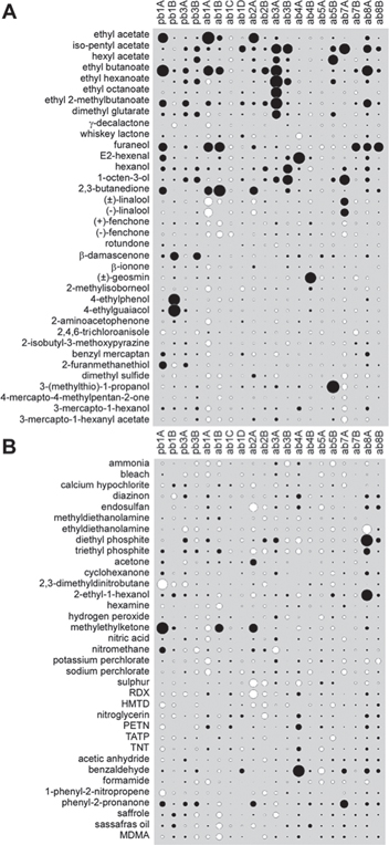
Figure 2. Responses of ORN classes to two disparate sets of volatiles. (A) Bubble plot of responses to a set of aroma chemicals from the wine industry, details are presented in supplementary table 1. Bubble area represents mean change in firing rate during stimulation (spikes/s). Actual values and SEM are in supplementary table 2. (B) Bubble plot of the same set of ORN classes to a set of volatiles related to security risks. Data are from Marshall et al (2009).
Download figure:
Standard image High-resolution imageNext we compared this response pattern to that observed across the same array of ORNs but to a much less natural set of volatiles (figure 2(B)). This set of mostly synthetic chemicals was assembled on the basis of representing a range of toxicity or security risks. We will refer to this set of odourants as the industrial set. At first sight it is obvious that the wine set evokes many more strong responses from the Drosophila receptors than the industrial set. For the latter, high responses (over 50 spikes/s) are only observed to a few of the compounds (9/35) though a few others evoke strong inhibitions (6/35). Nevertheless, at a threshold of 15 spikes/s many more are detected (21/35).
Testing the utility of Drosophila receptors for classification of odours
We then took the two sets of experimental data and asked how the selected ORNs would perform as sensors in a hypothetical artificial nose when tasked with classifying the chemicals in each of the two sets. Furthermore, we investigated how many and which of the ORNs should best be used for discriminating between the two different sets. In machine learning this problem is known as the feature selection problem, with the ORNs being the features.
To help us answer these questions we generated larger synthetic data sets, based on the experimental data (see methods), containing 20 simulated measurements for each of the 20 ORN × 71 chemical combinations, to enable a machine learning approach.
Computed classification performance for two odour sets is very similar
With these data we first addressed two related questions. Firstly, how many sensors should be grouped in an artificial nose to optimally recognize the odours within each of the two sets? Secondly, which specific sensors should be part of a nose of a given size. To address these questions we used a so-called wrapper-approach (Kohavi and John 1997), in which we generated all possible choices of groups of sensors. Each of these choices was used as the input space to a linear SVM and we inspected the classification performance in ten-fold cross-validation (see methods). Figure 3 (coloured bars in the centre) illustrates the overall results of this investigation. For both odour sets the best classification performance increases monotonically with the number of different sensors used. This seems intuitively obvious but is not necessarily always true; see (Nowotny et al 2013) for a counter-example from the domain of electronic noses. The best performance is reached when using all 20 available Drosophila receptor types but maximum performance, i.e. 100% with all volatiles recognized correctly at all times, was not observed even with the full set of sensors. However, performance increased quite rapidly with the number of sensors added to the nose so that 90% of the best observed performance (red line in figures 3(B), (C) is already achieved with 10 receptors for the industrial set and 11 receptors for the wine set.
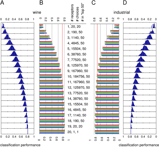
Figure 3. Classification performance of different groups of sensors for the two volatile sets (wine and industrial). (A) and (D): distribution of performance for all possible sensor group compositions for each given sensor group size (y axis). Labels in the middle indicate group size, total number of different groupings of this size and the number of groups in the 'top50' selection (see main text). (B) and (C): bar graphs of the best performance (dark red) and the average performance of the top50 selection (light red). Furthermore, the best performance of 'top50' members upon rerun of cross-validation (dark green) and the average performance of the 'top50' members in the rerun (light green). Finally, the best performance of 'top50' members in a rerun on a new synthetic data set (dark blue) and the average performance of 'top50' members in this rerun (light blue). The vertical red line marks 90% of the maximal performance observed overall.
Download figure:
Standard image High-resolution imageIt is possible that the reported best performance of certain groups of receptors was subject to a selection bias due to biased sampling of our synthetic data or bias in the selection of training and testing sets, for the replicated ten-fold cross-validations. To test for such bias we took the 50 best performing combinations of receptors for each nose size and independently performed ten more ten-fold cross-validations with them (figures 3(B), (C), green bars). If there had been chance bias in the selection of training and test sets, it would be unlikely to re-occur in exactly the same way and the observed performance in the second run should be markedly lower. However, the performance in the repeated cross-validation turned out to be very similar to the original values (wine set: difference of best −1.04 × 10⁻⁴ +/− 0.004, not significantly different from 0 (t-test, P = 0.91), difference of average top-50: −9.55 × 10⁻⁴ +/− 5.29 × 10⁻⁴, which is significantly different from 0 (t-test, P = 1.5 × 10⁻⁷); Industrial set: difference of best: −6.43 +/− 0.0033, not significantly different from 0 (t-test, P = 0.39), difference of average top-50: −0.001 +/− 0.001, significantly different from 0 (t-test, P = 2.9 × 10⁻⁴) suggesting that although there was a statistically significant selection bias for the average performance of the top-50 groups, it was of small overall magnitude for both of the two chemical sets.
To control for selection bias stemming from the particular generated synthetic data sets (see methods) we also repeated the analysis for the 50 best choices of receptor groups on an independently generated synthetic data set which had identical means and standard deviations to the original set (figure 3(B), C blue bars). The slight decrease in performance on average (compared to red bars) indicates a slight dependence of the choice of optimal sensor group on the particular synthetic data set used. (Differences between rerun and original run: Wine set: difference of best −0.0013 +/− 0.0134, not significantly different from 0 (t-test, P = 0.68), difference of average top-50: −0.013 +/− 0.0075, which is significantly different from 0 (t-test, P = 2.9×10⁻⁷; Industrial set: difference of best −0.0177 +/− 0.011, significantly different from 0 (t-test, P = 8.0 × 10⁻⁷), difference of average top-50: −0.029 +/− 0.012, significantly different from 0 (t-test, P = 2.4 × 10⁻⁹)). We note that the bias seems to be significantly larger for the industrial set than for the wine set, both for the for the best (ANOVA, P = 0.0001) and for the average top-50 (ANOVA, P = 1.5 × 10⁻⁵) performance difference between original and new synthetic data sets. However, compared to the overall variation between sensor groups of different size and between individual groupings of the same size, this bias is small.
Another aspect of the data displayed in figure 3 is the individual distributions of performance for each given size of the group of sensors used. The performance distributions exhibit much larger spread for small to medium group sizes than for larger group sizes, where the spread approaches zero. This indicates that the composition of the chosen group of sensors is crucial when only a few sensors are used, as one would expect, and becomes less important if a larger number of sensors is employed.
When comparing the performance of combinations of Drosophila sensors on the two different chemical sets, it is most striking that in spite of clear differences in the distribution of response magnitudes across ORNs and volatiles (figure 2) performance in classifying the odourants using these responses is quite comparable between the wine and industrial sets. Given this overall similarity we note that performance is slightly better on the industrial set than on the wine set when the nose is composed of single sensors, or small groups (<8). Conversely, the larger groups (9>) and the full set of 20 ORs perform slightly better on the wine set which is arguably more relevant to Drosophila behaviourally. One possible interpretation of this observation is that the industrial set may be more chemically diverse in terms of structures and physicochemical properties, like vapour pressure, and therefore easier to classify but the more complete sets of Drosophila ORNs may be better adapted to distinguish odours of the wine set.
Prevalence of ORN classes in the optimal sensor groupings differ for the two sets
Having addressed the questions of how groupings of sensors perform when used to recognize the chemicals in the two odour sets and how this performance depends on the group's size, we turn to a third question. Which individual sensors, on their own, are particularly successful in classifying each of the two sets or as part of an artificial nose of increasingly larger groupings of sensors? Put differently, if a nose contains only one sensor, which one will perform best? If it contains two, which sensors are best to combine? Furthermore, and particularly with groups of medium size, the optimal set of sensors for any group size need not contain the sensors that were part of the most successful group of fewer sensors.
Figure 4 shows that the ab8A receptor is one of the two most frequently chosen sensors in the most successful classifications of both wine and risk volatiles by single sensor noses (figure 4, panel 1). However, for the wine set receptor ab1A is overall the best sensor on its own (albeit at a poor performance of 11.4%) followed by ab8A (10.3% performance), while for the industrial set the best single OR is ab8A (14.7% performance) followed by pb1A (14.6% performance) as second best. For comparison, the chance levels for classification, i.e. the percentage of correct predictions expected if guessing any odour with equal probability of 1/36 or 1/35 respectively, are 2.8% for the wine set and 2.9% for the industrial set. The performance numbers for the single OR indicate that Drosophila ORs perform slightly better for the industrial set than for the wine set in this somewhat artificial challenge. A related but somewhat different question is which of the receptors is the most important if considering using all of them. One way of assessing this is to sequentially remove each OR from the full set of 20 considered here, to determine which one's removal leads to the largest decrease in classification performance. Inspecting the performance of the groups of 19 ORs reveals that the worst performing group for the wine set is the one missing receptor pb1B (75.5% compared to 81.7% with all 20 ORs) and, for the industrial set, the one missing receptor pb1A (73.9% compared to 78.5% with all 20 ORs).
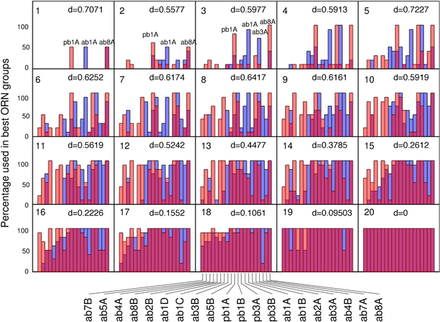
Figure 4. Comparison of the frequencies with which individual sensors appear in artificial noses of different sizes that lead to the best classifications of the two different odour sets (10% of all choices or 50 choices total, whichever is smaller, but at least one choice. Note that except for the single sensor case these are the top50 groups). The data was processed as in figure 3. The sensors were ordered on the horizontal axis according to the observed frequency of usage in the noses containing 16 sensors as used for classifying the wine set. Red bars correspond to the usage statistics for the industrial set and blue bars for the wine set. The purple colour marks their overlap. In each panel the number of receptors are noted in the upper left corner and the Hellinger distance between the histograms for wine and industrial sets are noted in the upper right corner.
Download figure:
Standard image High-resolution imageWhen comparing optimal choice of sensors, in particular for lower numbers, i.e., 1–12 sensors, we notice that different sensors are typically chosen for the two distinct odour sets. The amount of overlap in usage (shown in purple, figure 4) is generally smaller than the usage that is unique to either the wine or industrial set. To quantify this observation we calculated the Hellinger distance between the (normalized) histograms of receptor (sensor) use for the wine and industrial set for each of the receptor group sizes, i.e. each of the panels in figure 4. The results are noted in the panels. The Hellinger distance in principle varies from 0 (identical distributions) to 1 (maximally different distributions). Here, we observe zero distance for the group with all 20 sensors because in both cases all sensors are used, hence the distributions are identical. We observe maximal Hellinger distance for the group with 5 sensors, d = 0.723. Overall the calculation of Hellinger distance supports our impression, based on observing the plots in figure 4, that it is large for sensor choices with a small number of sensors and decreases to 0 for groups having most sensors. This indicates that, in agreement with our intuition, 'small noses' with only a handful of receptors would be very specialized, i.e. different for each specific application (specialist noses), and noses with many sensors would be similar to each other and hence might be useful for a number of different applications.
What role does the level of noise play?
In the case of Drosophila, multiple receptor neurons of the same type converge on the same glomerulus, with a convergence ratio of approximately 30:1 (Vosshall and Stocker 2007). This likely implies a noise reduction step due to averaging the noisy signals from individual receptor neurons. If the noise is fully independent between ORNs, we can expect a reduction of 1/√n, if n receptor neurons converge onto one local neuron or one projection neuron. Figure 5 illustrates the effect of reducing the sensor noise on the classification success. We reduced the standard deviation of the sensor responses in our generated data sets systematically from the full standard deviation, observed experimentally in single ORNs, in steps of 0.1 to 10% of this original value. For any number of sensors considered, the performance increases dramatically with decreasing noise and if using six or more receptor types, a reduction of the noise to 10% of its original value (corresponding to a convergence ratio of 100:1) already allows perfect performance of 100% recognition. For larger numbers of receptor types (ten or more) a reduction of the receptor noise to about 30% of its original value suffices to achieve 100% classification. When increasing noise levels, on the contrary, classification performance decreased monotonously with the noise level. This confirms that sensor noise is an important limiting factor for classification performance.

Figure 5. The effect of reducing or increasing the variability (noise) of the receptor neurons on the average performance of the previously identified top50 OR groups. The effects are similar for the wine (blue) and the industrial set (red). Reducing the noise dramatically improves classification performance and a reduction by a factor 10 (corresponding to a convergence ratio of 100:1 for independent ORNs) suffices in most cases (more than six receptors used) to achieve 100% classification performance. For small numbers of employed receptors, the industrial set appears to be classified slightly better while for large numbers of receptors the wine odours appear to be recognized better for all noise levels.
Download figure:
Standard image High-resolution imageWhich volatiles are easier to separate in each of the two sets and does this explain which sensors are picked?
We analysed how often each of the chemicals was recognized correctly and the frequency and nature of misclassifications.
Figure 6 illustrates the results for all feature set sizes from 1 to 20 receptors. It is clear that some odourants are usually recognized correctly by configurations that are not too small i.e. having more than four receptors. Most prominently, in the wine set, these are acetates, alkanoates and most alcohols (large black circles in figure 6). Also, for most of these well-classified chemicals, no other chemicals are confused with them (small or non-existent dark grey circles in figure 6). Other chemicals, however, are quite often recognized as something else, even for large feature set sizes, for example 4-mercapto-4-methylpentan-2-one, (+)-fenchone and (−)-fenchone, to name a few prominent examples in the wine set. This clear distinction demonstrates that there are objective differences in the separability of odourants, independent of the feature choices. The data for the industrial set show similar effects. Supplementary figures S1 to S4 show a more detailed analysis for the best feature sets. In these classification matrices we can recognize the nature of some of the typical errors in classification. For example, (±)-linalool and (−)-linalool, are—maybe not too surprisingly—quite frequently confused with each other but are rarely taken to be anything else and rarely is any other chemical mistaken to be one of them. A large group of odours, comprising approximately half of the chemicals, are misclassified as other odours quite frequently and other odours are frequently misidentified as being them. In this case the mistakes are spread among a larger group of analytes in both directions. This relationship between the two types of mistakes is, however, not necessarily symmetric. E.g. (−)-fenchone is frequently recognized to be γ-decalactone but γ-decalactone is rarely predicted to be (−)-fenchone. However, while strict symmetry is not observed, in most cases, when odour i is not misidentified as odour j (1131 occurrences for group size 20) then odour j is not misidentified as odour i (1100 occurrences for group size 20, i.e. in 97.3% of all cases, see supplementary figure S2). Similarly, if they are confused with each other in one direction (129 cases for group size 20), then they also tend to be confused the other way around (98 cases for group size 20, i.e. in 76% of all cases).
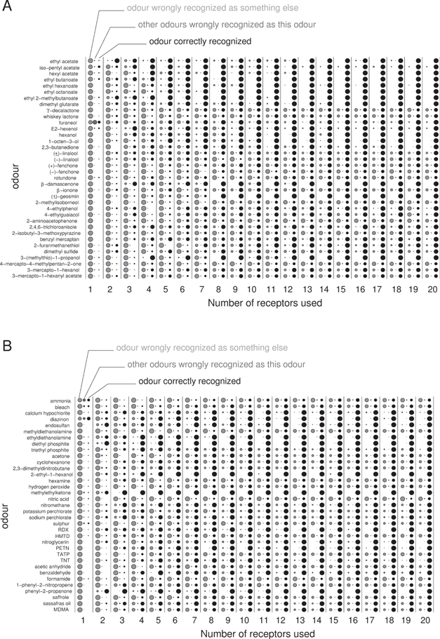
Figure 6. Summary of classification errors for the wine set (a) and the industrial set (b). The three columns for each e-nose size (number of used receptors) show how often each given odour was wrongly recognized to be a different chemical (light grey, left), how often another odour was erroneously recognized to be this odour (dark grey, middle), and how often the odour was recognized correctly (black, right). The area of the bullets is proportional to the fraction of occurrences of these events, normalized to the absolute maximum number with which they could occur. The values displayed are for the best observed choice of receptors for each e-nose size.
Download figure:
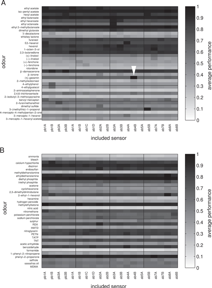
Standard image High-resolution imageFinally, we also investigated the question whether any individual receptors were particularly useful for recognizing specific odours. To quantify this we averaged the fraction of correct recognitions of each individual odour across all trials with feature sets that contained individual sensors. Figure 7 illustrates the results. Some odours, e.g. ethyl acetate, are always well-recognized, independent of the presence of individual receptors in the employed feature sets. Other odours, e.g. 4-mercapto-4-methylpentan-2-one, are consistently not well-recognized and the presence of none of the individual sensors seems to make a difference for the better or the worse. But there are also a few interesting cases, e.g. (±)-geosmin (white arrowhead on figure 7), that are not well recognized unless a particular receptor is employed (receptor ab4B for (±)-geosmin). Unsurprisingly ab4B is the receptor with the by far largest response to (±)-geosmin. The same correspondence applies to 3-(methylthio)-1-propanol and the ab5B receptor and to a lesser extent to 4-ethylphenol and 4-ethylguaiacol and the pb1B receptor. These more obvious examples seem to be predominantly found in the wine set, implying that they may be the result of specific evolutionary selection processes.
Figure 7. Average performance in recognizing individual odours, conditioned to whether individual sensors were present in the employed feature sets. (A) Wine set, (B) industrial set. For each pair of odour plus sensor, the grey level indicates the percentage of correct recognitions of the odour, averaged over all feature choices where the specified sensor was present.
Download figure:
Standard image High-resolution image
Despite these examples, it is worth noting that for most odours it is not straightforward to predict the relevance of receptors for their recognition this way. This perhaps explains why the Drosophila sensors do quite a reasonable job of classifying the industrial set. It is also worth noting that this analysis disregards false positives, i.e. it is not reflected in this analysis whether other odours may wrongly be classified as the odour under consideration in addition to the correct classifications of the odour that we report in figure 7.
Discussion
Our computational analysis reveals that subsets of Drosophila receptors appear surprisingly capable of distinguishing chemicals that they have not evolved to process, making their use in technical applications a realistic possibility.
Optimal e-nose size
We find that, in contrast to our recent work with metal oxide sensors (Nowotny et al 2013), where medium-sized sensor arrays performed best, chemical sensing with Drosophila receptors appears to achieve the best recognition accuracy for both the wine set (81.5%) and the industrial set (77.6%) if the outputs of all 20 OR types are used. One possible reason for this difference could lie in the fact that biological olfactory receptors appear to be less correlated in their responses (both in insects (Berna et al 2009) and mammals (Fonollosa et al 2012)) than metal oxide sensors. However, 90% of the performance (73.4% and 69.8% correct classification respectively) of all 20 OR types can be achieved by an appropriately chosen subset of as few as 10–11 receptor types. This compares with the chance probabilities of correctly classifying any given sample, which are 2.8–2.9%. We also found that, if such smaller subsets of sensors are used, the best choices tend to be specific to the individual problem, i.e. the optimal sensor choices for the wine set and industrial set differed most for medium-sized e-noses. The membership of the sets of most relevant receptors for discriminating within wine and industrial sets therefore overlap but are not identical.
Interestingly, if only very few receptor types are utilized, Drosophila ORs distinguish the industrial set chemicals significantly better than those of the arguably behaviourally more relevant wine set. If all 20 receptor types are included, however, the situation is reversed and the wine set is classified better. This may follow from the principle that species with larger numbers of receptor types may be capable of higher levels of olfactory resolution among a common set of odourants as much as broadened receptivity to novel odourant classes.
Noise
The data used in this work are from in vivo recordings of Drosophila sensilla on the antennae and maxillary palp. The recordings are influenced by several sources of noise and variability: Odour concentrations in the delivery system may vary slightly and some neurons may be affected by the insertion of a saline-filled electrode in the vicinity. The recordings from different sensilla within the same animal vary due to electrode placement and the natural biological variability of the sensilla and the ORNs within them. And, finally, the ORNs from different animals vary, genetically, developmentally and due to recent experience. We have here lumped all variability and noise into the standard deviation of the responses of different ORs and resampled Gaussian distributions with this standard deviation. We envisage that, in a technical application using isolated ORs from Drosophila, some of the variability and noise we encounter would be less than our current conservatively large observations. In order to estimate the sensitivity of the classification performance to such diminishing variability, we retested our algorithms with resampled data sets having reduced noise. These numerical experiments elucidate the improvement in odour recognition that could be achieved if the noise in all receptors were reduced, e.g. by linear superposition of several olfactory receptor neuron responses, as presumably occurs in the glomeruli of the antennal lobe. Our results indicate that a convergence of 100:1 (i.e. ten-fold reduction of standard deviation) would be sufficient to give perfect classification performance for the tasks envisaged here. If similar reductions in noise could be achieved in a technical solution, we would expect such an e-nose to be able to faultlessly recognize the chemicals in either the wine set or the industrial set at the fixed concentrations used here.
Concentrations and limited number of chemicals
Real world problems as they are experienced by animals or presented to an electronic nose, usually require classification of odours or mixtures of odours independent of their concentration, at least over quite a wide range of concentrations. This is a level of complexity we did not attempt to replicate in this study, largely because of the level of resources that would be required to collect meaningful, replicated, data. In our study each odourant is considered a unique entity and stimulates each neuron independently. Varying an odourant's concentration (intensity) would vary the responses across the array of sensors in a correlated way, adding an extra, quite different, layer of complexity. Dose-response relationships of Drosophila receptors are reliably sigmoid shaped with a dynamic range of 2–3 decadic steps (de Bruyne et al 2001, Mathew et al 2013). Variability for a particular neuronal class is relatively small, typically less than one decadic step, which is considerably lower than that observed in mice (Grossmaitre et al 2006). Consequently, for odourants evoking responses between 20–200 spikes/s at the concentrations we tested the dose-reponse relationship is reasonably predictable. For odourants outside this range it is harder to predict how far concentrations have to be lowered or raised for the response to fall within this dynamic range. Hallem and Carlson (2006) showed how odourants at concentrations evoking saturated response levels above 200 spikes/s, 'drop out' of the response profile when they are diluted a further 2 or 4 decadic steps, undoubtedly making classification harder. In addition, in real world applications, odourants may be encountered against a background of many more chemicals than we were able to include in the two sets used here. The accuracies of classification reported in this study should therefore not be construed to be direct predictions of a hypothetical Drosophila OR based e-nose in any particular practical application. Nevertheless even classifying 71 chemicals, each at a fixed concentration, is a challenging problem, particularly compared with what is generally attempted in machine olfaction studies. Further work is certainly needed to address the issue of feature selection and classification when odour concentrations are varied.
General validity and relevance of the results
Although the odour stimuli used and the responses recorded in this study are genuine, we do not claim that the resampled responses are necessarily a faithful reflection of what the fly experiences in vivo. Nevertheless, this study is probably the first attempt to assemble a large matrix of odour-receptor responses with sufficient replication to begin the task of selecting informative features and comparing their classification performance, quantitatively across odour sets and qualitatively with engineered sensor arrays. The choice of a SVM to perform classification was largely based on considerations of convenience, as it is well-known in the field, easily implemented in the wrapper approach and, importantly, allows direct comparisons with earlier work on feature selection and classification of volatile odours, using metal oxide sensors (Nowotny et al 2013). To exclude any artefacts originating from this particular choice, we have repeated our classification assessments with two other common classifiers, a centroid classifier and a k-nearest neighbours (kNN) classifier (figures S6–S10). While we can see minor differences, typically in that centroid and kNN classifiers outperform on a smaller number of features and SVM is slightly better for large numbers of features, the differences are so small that using a different classifier would not change the conclusions we arrived at using the linear SVM classifiers above.
It is clear from our earlier work (Nowotny et al 2013) and this current study that the concept of a bioelectronic nose being used to classify a range of chemicals that have not featured in the evolution of the sensors is reasonable. Although, unlike in the case with metal oxide sensors (Nowotny et al 2013), classification performance improves monotonically with the number of ORN sensor types used, quite good classifications can be achieved using small numbers of sensors. Related work with artificial neural networks (Bachtiar et al 2013) predicting the chemical class of odourants based on previously published Drosophila OR response data (Hallem and Carlson 2006) found a similar effect, where 15 out of 20 receptors appeared to be the optimal number for classification. The fact that subsets of sensors can be selected to perform particular tasks is also encouraging for attempts to actually build a bioelectronic nose. However, despite the acceptable performance of the Drosophila receptors in classifying industrial chemicals, the finding that strong matching between an individual receptor and a target chemical, e.g. ab4B and geosmin, is restricted to the wine set, suggests that selective re-engineering of the specificity of a small number of naturally evolved receptors might yet still improve the performance of the whole.
Acknowledgements
Markus Herderich of the Australian Wine Research Institute for provision of rotundone. This work was supported by CSIRO Flagship Collaboration Fund and the EPSRC (grant number EP/J019690/1). We thank Drs David Lovell and David Clifford for critical reading of the manuscript.