Abstract
Estimates based on the strength, size, and shape of the Atlantic razor clam (Ensis directus) indicate that the animal's burrow depth should be physically limited to a few centimeters; yet razor clams can dig as deep as 70 cm. By measuring soil deformations around burrowing E. directus, we have found the animal reduces drag by contracting its valves to initially fail, and then fluidize, the surrounding substrate. The characteristic contraction time to achieve fluidization can be calculated directly from soil properties. The geometry of the fluidized zone is dictated by two commonly-measured geotechnical parameters: coefficient of lateral earth pressure and friction angle. Calculations using full ranges for both parameters indicate that the fluidized zone is a local effect, occurring between 1–5 body radii away from the animal. The energy associated with motion through fluidized substrate—characterized by a depth-independent density and viscosity—scales linearly with depth. In contrast, moving through static soil requires energy that scales with depth squared. For E. directus, this translates to a 10X reduction in the energy required to reach observed burrow depths. For engineers, localized fluidization offers a mechanically simple and purely kinematic method to dramatically reduce energy costs associated with digging. This concept is demonstrated with RoboClam, an E. directus-inspired robot. Using a genetic algorithm to find optimal digging kinematics, RoboClam has achieved localized fluidization burrowing performance comparable to that of the animal, with a linear energy-depth relationship, in both idealized granular glass beads and E. directus' native cohesive mudflat habitat.
Export citation and abstract BibTeX RIS

Content from this work may be used under the terms of the Creative Commons Attribution 3.0 licence. Any further distribution of this work must maintain attribution to the author(s) and the title of the work, journal citation and DOI.
1. Introduction
Burrowing in soil presents challenges in engineering and biological applications alike. Many animals have developed unique locomotion schemes to move through particulate substrates [1]. The sandfish lizard (S. scincus) undulates in the manner of a fish in order to effectively swim through sand [2]. Clam worms (N. virens) have been observed to use crack propagation to burrow in gelatin, a material with similar properties to elastic muds [3]. Smaller organisms, like nematodes (C. elegans), have been observed to move efficiently via reciprocating motion in saturated granular media [4, 5].
Contrary to a generalized Newtonian fluid, in which viscosity and density do not change with depth, particles within a static granular material experience contact stresses, and thus frictional forces, that scale with the surrounding pressure, resulting in shear strength that increases linearly with depth [6]. This means that submerging devices such as anchors and piles can be costly, as insertion force F(z), increases linearly with depth z [7], resulting in an insertion energy, E = ∫F(z) dz, that scales with depth squared.
Ensis directus, the Atlantic razor clam, can produce a force of approximately 10 N to pull its valves into soil [8]. Using measurements from a blunt body the size and shape of E. directus pushed into the animal's habitat substrate, we determined that this much force should enable the clam to submerge to approximately 1–2 cm [9]. But in reality, razor clams dig to 70 cm [10]3, indicating that the animal must manipulate surrounding soil to reduce burrowing drag and the energy required for submersion.
E. directus burrows by using a series of valve and foot motions to draw itself into underwater soils (figures 1(A)–(E)). An upper bound of the mechanical energy associated with advancing its valves downward can be estimated by adapting results from Trueman [8], who measured the following biomechanical parameters of E. directus digging in sand: pulling forces between the valves and foot, valve contraction angles, the pressure developed between the valves during contraction, and the torsional stiffness of the valve ligament. Summing the energies and kinematics associated with motion of the valves during one burrow cycle yields: valve uplift (0.05 J, −0.5 cm), valve contraction (0.07 J, 0 cm), and valve penetration (0.20 J, 2.0 cm), combine for a total of 0.21 J cm−1 (with positive displacements relating to downwards progress into the soil). Re-expansion of the valves is accomplished through elastic rebound of the hinge ligament, and thus requires no additional energy input by the animal. Comparing this performance to the energy required to push an E. directus-shaped blunt body to burrow depth in the animal's habitat substrate using steady downward force (figure 1(F)), we find the animal is able to reduce its required burrowing energy by an order of magnitude, even though there is an energetic cost associated with pushing up and contracting its valves—motions that do not directly contribute to downward progress.

Figure 1. E. directus digging cycle kinematics and energetics. Dashed line in (A)–(E) denotes a depth datum. White arrows indicate valve movements. Red silhouette denotes valve geometry in expanded state, before contraction. (A) Extension of foot at initiation of digging cycle. (B) Valve uplift. (C) Valve contraction, which pushes blood into the foot, expanding it to serve as a terminal anchor. (D) Retraction of foot and downwards pull on the valves. (E) Valve expansion, reset for next digging cycle. (F) Energetic cost to reach burrow depth for E. directus and a blunt body of the same size and shape as the animal pushed into static soil. Inset (a) shows the kinematics and energetics corresponding to (A)–(E). E. directus data adapted from [8]. Blunt body data collected from 15 penetration tests in real E. directus habitat off the coast of Gloucester, MA. Error bars denote ± STDEV.
Download figure:
Standard image High-resolution imageWe have found that the uplift and contraction motions of E. directus' valves during burrowing locally agitate the soil (figure 2(A)) and create a region of fluidization around the animal [9]. Moving through fluidized, rather than static, soil reduces drag forces on the animal to within its strength capabilities [9]. These fluidized substrates can, to first order, be modeled as a generalized Newtonian fluid with depth-independent density and viscosity that are functions of the local packing fraction [11–16].
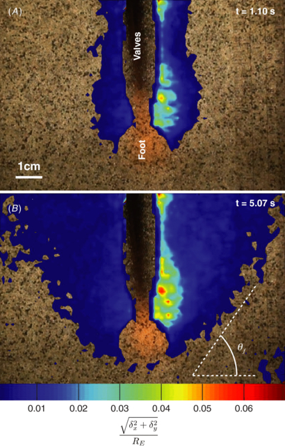
Figure 2. Soil movement around burrowing E. directus. Horizontal and vertical displacement fields from PIV data, δx and δy, respectively, are plotted together as displacement magnitude, non-dimensionalized by the initial radius of E. directus, RE. Data are overlaid on original video frames used for PIV. The animal's body is masked from the data. The color bar spans 0.001–0.07. (A) Completion of valve uplift and contraction (1.10 s after initiating burrowing cycle), showing the fluidized zone proximate to the animal's body. (B) Moment when soil failure wedge fully forms, occurring after retraction of foot and downward pull on valves (5.07 s after initiating burrowing cycle). The predicted failure wedge angle, θf, is calculated from the substrate friction angle and is shown with a white dashed line.
Download figure:
Standard image High-resolution imageE. directus is an attractive candidate for biomimicry when judged in engineering terms: its body is large (approximately 20 cm long, 3 cm wide); its shell is a rigid enclosure with a one degree of freedom hinge; it can burrow over half a kilometer using the energy in an AA battery [17]; it can dig quickly, up to 1 cm s−1 [8], and it uses a purely kinematic event to achieve localized fluidization, rather than requiring additional water pumped into the soil. There are numerous industrial applications that could benefit from a compact, low-energy, reversible burrowing system, such as anchoring, subsea cable installation, mine neutralization, and oil recovery. An E. directus-based anchor should be able to provide more than ten times the anchoring force per insertion energy as existing products [18].
This paper presents the mechanics that govern localized fluidization burrowing and experimental validation that E. directus-inspired digging can be transferred to engineering applications. Timescales and formation of the fluidized zone are derived from soil, fluid, and solid mechanics theory. This analysis indicates that localized fluidization burrowing is possible in cohesive and granular soils, and that the size of the fluidized zone can be predicted from commonly measured geotechnical parameters. Using RoboClam, an E. directus-inspired robot that learns to dig efficiently using a genetic algorithm (GA), we demonstrate that a machine can achieve comparable digging performance to the animal, with borrowing energy scaling linearly with depth in an idealized granular substrate and E. directus' habitat—cohesive mudflat soil. These experiments also validate the critical valve contraction timescale to achieve fluidization, which can be predicted from soil parameters.
2. Mechanics of localized fluidization burrowing
2.1. Initiating fluidization
The adage 'clear as mud' is often used to describe the difficulty of visually investigating burrowing animals in situ. To explore the soil mechanics at play during E. directus burrowing, we constructed a 2D ant farm, or Hele-Shaw cell [19], to see through the substrate surrounding a digging animal and measure deformation of the granular medium with particle image velocimetry (PIV) [9]. This work showed that the uplift and contraction motions of E. directus' valves agitate the surrounding soil (figure 2(A)), creating a state of localized fluidization. This event occurs at a faster timescale than that required for the soil to naturally fail and landslide toward the animal (figure 2(B)).
The discontinuity at the failure surface, shown by θf in figure 2(B), enables fluidization to occur—as the valves contract beyond the point when incipient failure is induced in the soil, the particles in the failure zone are free to move with the pore fluid while the particles outside the failure zone remain stationary. The relevant Reynolds number of the pore fluid flow,  , calculated from E. directus' valve velocity vv (determined from the valve contraction angular velocity and valve width), particle diameter dp, and the pore fluid density ρf and viscosity μf, varies between 0.02 and 56, depending on particle size (0.002–2 mm [6, 8, 10]), animal size (10–20 cm, from experimental observation), and valve contraction velocity (vv ≈ 0.011–0.028 m s−1 [8]). As this range of Reynolds numbers falls primarily within the regime of Stokes drag (the transition to form drag occurs at a Reynolds number of approximately 100) [20], the characteristic time for a particle to reach the pore fluid velocity can be estimated through conservation of momentum:
where mp is the mass of a soil particle,  is the acceleration of the particle, and ρp is the density of the particle. For the 1 mm soda lime glass beads used in our experiments, tchar = 0.075 s. This timescale is considerably less than the ≈ 0.2 s valve contraction time measured by Trueman [8], indicating that soil particles surrounding E. directus can be considered inertialess and are advected with the pore fluid during valve contraction.
The discontinuity created by the failure surface is critical to achieving fluidization, as without it substrate particles would follow the fluid flow field, which is incompressible and governed by  . No divergence in the flow field creates no divergence between particles, and thus no unpacking. However, in the presence of a finite failure zone, E. directus' contraction motion reduces the volume between the valves, which draws pore water into the region surrounding the animal. This pore water mixes with the failed soil to create a locally unpacked, fluidized zone.
2.2. Localized substrate failure during valve contraction
The previous subsection relates to our measurements of E. directus in a two-dimensional experimental setup; the following discussion is focused on describing the mechanics that govern how the failure, and fluidized, zone forms around the animal in three dimensions.
As E. directus initiates contraction of its valves, it reduces the level of stress acting between the valves and the surrounding substrate, causing failure in the soil. Figure 3(A) shows a Mohr's circle representation [21] of the effective stress states at equilibrium, before contraction (circle a), and during the initiation of contraction, which brings the soil to one of two states of active failure, caused either by an imbalance between radial and vertical stresses (circle b), or an imbalance between radial and hoop stresses (circle c). Effective stress is the actual stress acting between soil particles, neglecting hydrostatic pressure of the pore fluid, and is denoted in this paper with a prime. The term 'active' corresponds to the reduction (rather than increase) of one of the principal stresses to induce failure [6].
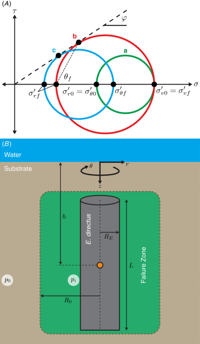
Figure 3. Soil failure mechanisms around burrowing E. directus in 3D. (A) Mohr's circle showing stress states at equilibrium (a), failure due to radial–vertical stress imbalance (b), and failure due to radial–hoop stress imbalance (c). Labels: τ is shear stress; σ is normal stress; φ is the soil's friction angle; θf is the predicted failure angle; superscript ' denotes effective stress, the actual stress between substrate particles without the contribution of pore water hydrostatic pressure; subscript r denotes radial direction; subscript v denotes vertical direction; subscript θ denotes hoop direction; subscript 0 indicates equilibrium state; and subscript f indicates failure state. (B) Schematic of the failure zone in soil around contracting E. directus. Labels: p0 is equilibrium lateral soil pressure; pi is the soil pressure acting on the animal's valves; r, z, and θ denote the cylindrical coordinate system; h is E. directus' depth in the substrate; L and R0 are the animal's length and expanded radius, respectively; and Rf is the radius of the failure zone.
Download figure:
Standard image High-resolution imageAs the soil begins to fail, it will tend to naturally landslide downward at a failure angle θf. At this point, the shear stresses in the soil are equal to its shear strength. This condition is shown in figure 3(A), with the applied stress circles b and c tangent to the failure envelope, which lies at the same angle as the friction angle of the soil φ, a property commonly measured during a geotechnical survey. The failure angle is the transformation angle between the principal stress state and the stress state at failure. This angle can also be determined by connecting the tangency point on the failure envelope, the horizontal effective stress at failure  , and the principal stress axis (figure 3(A)), and is given by
Equation (2) was used to plot the failure angle in figure 2(B), with the friction angle of the substrate measured as 25°.
To describe soil failure in three dimensions, we propose a simplified model of E. directus as a cylinder with contracting radius that is embedded in saturated soil (figure 3(B)). To neglect end effects, the length of the cylinder is considered to be much larger than its radius. When E. directus initiates valve contraction, it induces incipient failure without moving the substrate particles; as this relaxation in pressure can be considered quasi-static and elastic [6], stresses due to inertial effects can be ignored and the total radial and hoop stress distribution in the substrate can be described with the following thick-walled pressure vessel equations [22], which have been modified to geotechnical conventions (with compressive stresses positive) and to reflect an infinite soil bed in lateral directions:
where σr is total radial stress, σθ is total hoop stress, R0 is E. directus' expanded radius (before contraction), pi is the pressure acting on the animal's valves, and p0 is the natural lateral equilibrium pressure in the soil. It is important to note that these equations still hold if there is a body force acting in the z-direction, such as in soil. In this case, the pressure vessel equations describe the state of stress within annular differential elements stacked in the z-direction. The total vertical stress is given as

where h is the clam's depth beneath the surface of the soil, ρt is the total density of the substrate (including solids and fluids), and g is the gravitational constant. It should be noted that there are no shear stresses within the soil in principal orientation, as τrz = τθz = 0 because E. directus is modeled with a high aspect ratio (L ≫ R0) and τrθ = 0 because of symmetrical radial contraction.
The undisturbed horizontal effective stress in the substrate is determined by subtracting hydrostatic pore pressure u from the natural lateral equilibrium pressure:

The undisturbed horizontal and vertical effective stresses can be correlated through the coefficient of lateral earth pressure
which is a soil property that can be measured through geotechnical surveys [6, 23]. By also knowing the void fraction of the soil  and the particle and fluid density, ρp and ρf respectively, p0 can be determined as

Failure of the substrate will occur when pi is lowered to a point where the imbalance of two principal effective stresses produces a resolved shear stress that equals the shear strength of the soil. This resolved failure shear stress can be created by an imbalance between radial and vertical stresses (figure 3(A), circle b) or radial and hoop stresses (figure 3(A), circle c). From the geometry of either circle and the failure envelope defined by φ, the relationship between stresses at failure for either mechanism is
where the subscript f denotes the stresses at failure and Ka is referred to as the coefficient of active failure. It is important to note that this failure analysis is also valid for cohesive soils. The difference between cohesive and granular soils when plotted on a Mohr's circle is that the failure envelope does not pass through (0,0), as cohesive stresses give soil shear strength even when no compressive stresses are applied. At sufficient depths the failure envelope can be approximated as running through (0,0) for any soil type, as compressive stresses due to gravity will dominate cohesive stresses.
Soil failure due to an imbalance between radial and vertical stresses will occur when the applied radial effective stress equals the radial stress at failure. The radial location of the failure surface in this condition,  , can be found by combining (3) for radial stress with (6), (7), and (9), and realizing that the vertical effective stress at failure and equilibrium is unchanged, namely
yielding the dimensionless radius for radial–vertical stress imbalance-induced failure:
If soil failure is caused by an imbalance between radial and hoop stresses, the radial location of the failure surface,  , can be found by combining (3) and (4) with (6) and (9):
yielding the dimensionless radius for radial–hoop stress imbalance-induced failure:
The dominant failure mechanism in the soil surrounding a contracting cylindrical body is determined by the type of failure (radial–vertical or radial–hoop) that results in the largest failure surface radius. The ratio of failure radii for both mechanisms can be calculated by combining (10) and (11) into
Figure 4(A) shows values of (12) for the full range of possible soil types, with 0.19 ⩽ Ka ⩽ 0.52 and 0.31 ⩽ K0 ⩽ 1 [6, 23]. For the region of radial–hoop stress-dominated failure (above the dashed line in figure 4(A)),  , indicating that the failure radius from both mechanisms is approximately the same size. For the region of radial–vertical stress-dominated failure (below the dashed line in figure 4(A)),
  and rapidly rises to an asymptote for lower values of K0 and higher values of Ka. The asymptote and the imaginary region in figure 4(A) correspond to natural stress imbalances that exceed the shear strength of the soil and are thus impossible. Since
  , radial–vertical stress imbalance-induced failure is considered the dominant mechanism and is used to predict the failure zone size from the following scaling arguments.
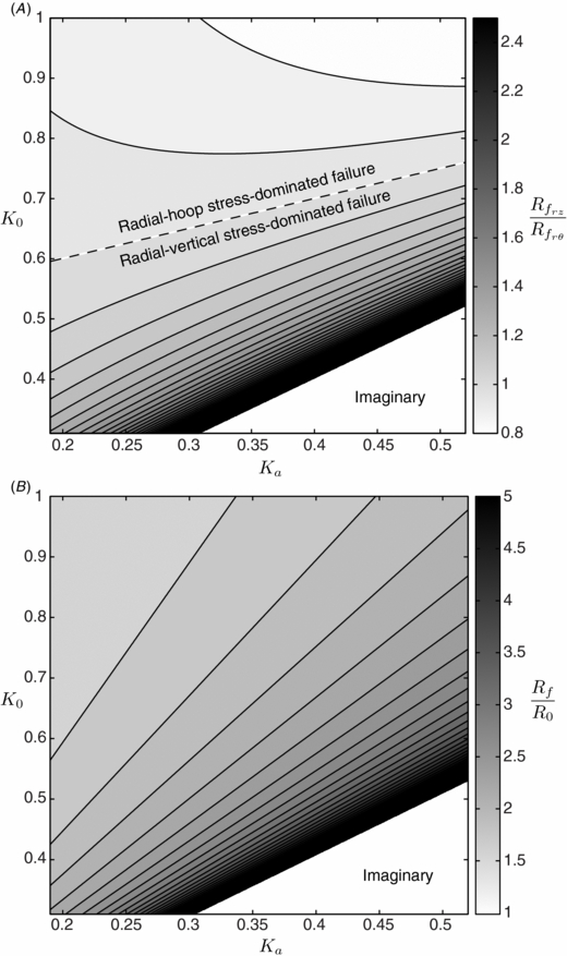
Figure 4. Size of soil failure zone around contracting E. directus. (A) Ratio of predicted failure zone radii due to radial–vertical stress imbalance,  , and radial–hoop stress imbalance,
  . Dashed line shows
  . (B) Generalized failure radius, Rf, non-dimensionalized by E. directus' radius, R0, predicted using equation (13). Both (A) and (B) are plotted for all possible soil types, characterized by coefficient of lateral earth pressure, K0, and coefficient of active failure, Ka. Imaginary regions in both plots correspond to impossible stress states, where the soil is not strong enough to carry such a large imbalance between horizontal and vertical stresses.
Download figure:
Standard image High-resolution imageIf during contraction pi is assumed to be approximately zero, corresponding to complete stress release between E. directus' valves and the surrounding soil, and u ≈ 0.5p0 because of the relative densities and volumetric fractions of the soil particles and interstitial water, (10) reduces to
This facilitates a prediction of Rf using only two soil properties, Ka and K0, both of which are commonly measured during a geotechnical survey [24].
Applying the range of possible Ka and K0 values to (13) yields  in most conditions (figure 4(B)). These results demonstrate that soil failure around a contracting cylindrical body is a relatively local effect, and for reductions of pi to near zero, depth-independent. Equation (13) also does not depend on any soil cohesion terms, indicating that localized substrate failure and fluidization should be possible in both granular and cohesive soils.
3. Materials and methods
3.1. Design of RoboClam
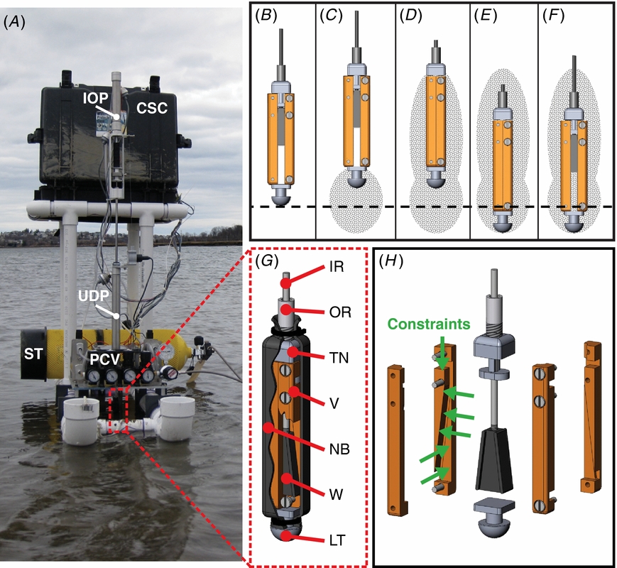
To explore the transfer of localized fluidization burrowing to engineering applications, we designed and built RoboClam, a robot that replicates the digging kinematics of E. directus (figure 5(A)). The robot consists of a control platform with two pneumatic pistons that actuate an end effector in the same up-in-down-out motions as E. directus' valves (figures 5(B)–(F)). The end effector is the same size scale as E. directus (9.97 cm long and 1.52 cm wide) and is capable of the same contraction displacement of an adult animal (∼6.4 mm). Unlike E. directus, which uses its foot—a soft, dexterous organ—to move its valves up and down, RoboClam uses a simpler mechanical arrangement to actuate the end effector up and down with a pneumatic piston, which is capable of a much longer stroke than the animal's foot. Pneumatics were chosen as the main power source so RoboClam can be safely tested in real, undisturbed ocean substrates, which enables accurate comparisons to E. directus performance and mitigates container wall effects.
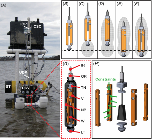
Figure 5. Anatomy of the RoboClam. (A) RoboClam burrowing in E. directus habitat on a mudflat in Gloucester, MA. Dashed line box shows location of the end effector. The in-out piston (IOP) and up-down piston (UDP) control in-out and up-down motions of the end effector, respectively. The robot runs on compressed air from a scuba tank (ST), regulated by pressure control valves (PCV). Measurement and control is accomplished by a laptop housed in the control system case (CSC). (B)–(F) Motions of the end effector while burrowing, which replicate E. directus' valve motions (figures 1(A)–(E)). Dashed line indicates depth datum. Shaded areas show regions of anticipated localized fluidization. (G) Sectioned view of the end effector mechanism. The inner rod (IR) actuates in-out motion and the outer rod (OR) actuates up-down motion of the end effector. The top nut (TN) vertically constrains the two valves (V). The neoprene boot (NB) prevents soil particles from jamming the mechanism. The wedge (W) slides up and down to force the valves in and out. The leading tip (LT) bears the majority of abrasive forces from downwards motion instead of the boot. (H) Exploded view of the end effector showing contact points between the wedge, valves, and top nut, which provide six constraints (green arrows) to exactly constrain the mechanism.
Download figure:
Standard image High-resolution imageThe end effector is sealed within a rubber boot to prevent soil particles from jamming the valve expansion/contraction mechanism (figure 5(G)). Displacement of the mechanism is accomplished with a sliding wedge that moves the two valves of the end effector in and out. The wedge and valves are exactly constrained (figure 5(H)), with contact lengths/widths greater than two in order to prohibit jamming during any part of the stroke [25]. The wedge was designed to intersect the center of pressure of the valves regardless of its position, assuming the center of pressure is located approximately at the center of the valves. The geometry and exact constraint of the end effector mechanism allow its efficiency to be characterized by measuring the coefficient of friction between the wedge and valves, which was found to be 39% [26].
As RoboClam burrows, the control system tracks the total amount of energy input to the system by integrating the forces acting on the pneumatic actuators over their displacement. Because we were able to characterize the frictional losses in the end effector and the actuators, as well as account for potential energy changes, the energy expended for soil deformation while burrowing could be tracked [26]. This is an important facet of the machine's design, as overall energy consumed is device-dependent; the purpose of creating RoboClam was to test the new method of using a machine to burrow via localized fluidization. After the method is understood and characterized, other burrowing machines can be designed for optimized efficiency.
3.2. RoboClam testing
RoboClam is controlled using a GA. The control space for the robot is composed of eight independent parameters: up/in/down/out pneumatic pressure and the time or displacement associated with each motion. A GA was used because it can handle many independent variables in an optimization problem. The random mutation and recombination of traits used by a GA may allow it to find a global minimum, even in situations in which other optimization methods would not [27]. During the ocean tests reported in this work, MATLAB's4 built-in GA was used, with a population of 10–20 individuals running for 10–20 generations. In laboratory tests reported, RoboClam ran from customized GA software written in Python5.
A GA is analogous to evolution in nature [27]. In the case of RoboClam, the GA begins a test by randomly generating a population of individuals, where each individual is a set of instructions (movement times/displacements and pressures) to run the machine. The GA runs the robot with each individual and records its digging performance. Individuals are then compared by a metric to be optimized—a 'cost' function that relates to digging efficiency for RoboClam. Individuals in the population with the lowest cost are allowed to interbreed (mix parameters) with each other, high-cost individuals are killed off, and new individuals are added to the population to form the next generation. The process repeats for many generations, ideally continually decreasing the cost to a global minimum, which appears as a cost asymptote.
In quantifying optimized burrowing efficiency, two factors are relevant: the overall energy expenditure per depth of the robot β, where  ; and the power law relationship α between energy expended and depth, where
  with the energy-depth data centered about (0, 0). Fluidized soil exhibits α = 1, whereas static soil exhibits α = 2. The cost function used for the first set of tests reported in this work (figure 6) was

These tests were conducted in real E. directus habitat off the coast of Gloucester, MA. One hundred and twenty five tests were run during the trial, representing 13 generations of the GA (with the final generation incomplete). The controlled digging parameters were up and down time, in and out displacement, and the pressures associated with each movement. The robot was moved to a new location for each test, greater than ten characteristic lengths away from the previous test, as to maintain virgin soil conditions.
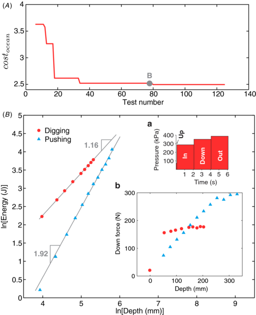
Figure 6. RoboClam burrowing data from ocean mudflat testing in Gloucester, MA. (A) Minimum value of costocean for each generation of the genetic algorithm controlling RoboClam (125 individual tests). Point B corresponds to the lowest cost test with α ≈ 1, where α is the power law relationship between burrowing energy and depth. (B) Test data from point B in (A), with digging data from RoboClam. Pushing data is from the E. directus-shaped blunt body in figure 1, taken at the same location. Inset (a) commands for actuation pressure and duration given to the robot during the test. Inset (b) applied downward force versus depth for RoboClam digging and blunt body pushing.
Download figure:
Standard image High-resolution imageWe found that low values of β resulted in low-energy burrowing for depths of 20–30 cm, but with relatively high α (≈2, indicating non-fluidized substrate). At greater depths these burrowing techniques would not provide any energetic advantage over existing techniques used to penetrate static soil [7]. As a result, the cost function used for the second set of data reported in this work (figure 7) was

as α ≈ 1 demonstrates localized fluidization—the aim of our experiments. These tests were conducted in 1 mm soda lime glass beads saturated with water, the same substrate used in our visualization experiments of E. directus. The beads were contained in a 0.125 m3 (33 gallon) steel drum with the robot mounted on top. The diameter of the drum was greater than 10X the width of the end effector. Three hundred and seventy one individual tests, constituting ten separate trials, were performed with this setup and are reported in this work.
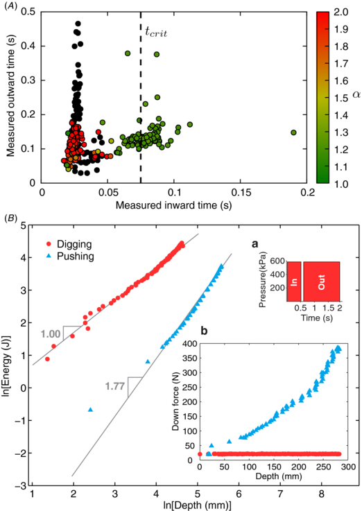
Figure 7. RoboClam testing in 1 mm soda lime glass beads. (A) Power law relationship α between burrowing energy and depth, dependent on actual contraction and expansion times of the end effector. Digging tests run with only in/out actuation of the end effector, with the robot falling under its own weight. Values of α ≈ 1 denote burrowing via localized fluidization; values of α ≈ 2 indicate no fluidization and static soil. Black dots are tests where burrowing depth was less than one body length and deemed unsuccessful. Critical contraction time to achieve fluidization, tcrit, matches the advection time for particles to reach pore fluid flow velocity during contraction, determined by (1). Data from 362 individual tests collected during 18 trials. (B) RoboClam digging test with lowest α from (A), compared against the end effector pushed into static substrate without actuating the in/out motion. Inset (a) commands for in/out actuation pressure and time given to the robot during the test. Inset (b) applied downward force versus depth for RoboClam digging versus pushing.
Download figure:
Standard image High-resolution image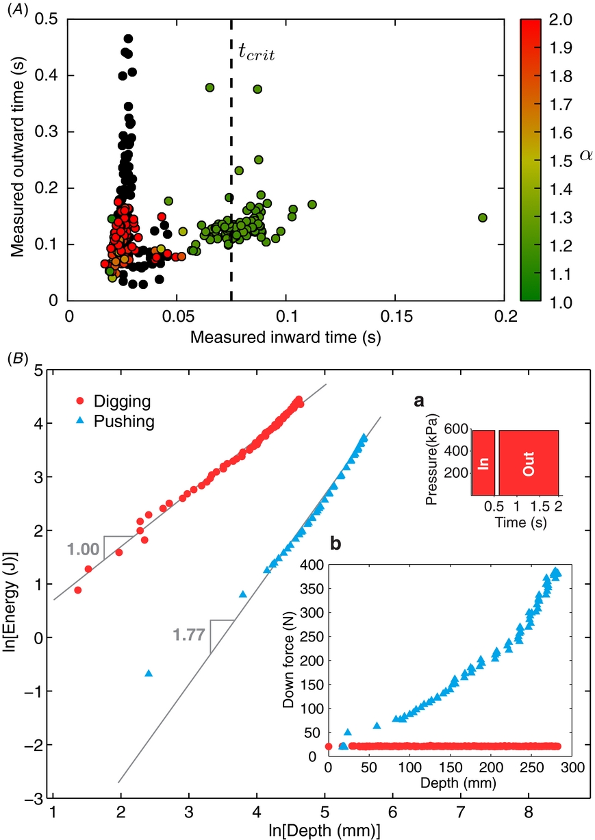
4. Results and discussion
Figure 6(A) shows how RoboClam evolved toward improved digging performance in the ocean mudflat through each generation of the GA, with costocean hitting a plateau for latter tests. Point B corresponds to the test parameters given in figure 6(B), which was the lowest cost test of the trial that had α ≈ 1; values of costocean in figure 6(A) that are slightly lower than point B correspond to tests where β was low but α ≈ 2, indicating no localized fluidization. The power law relationship between energy and depth in figure 6(B) shows that RoboClam achieved localized fluidization by using E. directus burrowing motions (inset a), which also resulted in a nearly constant downward force (inset b); in contrast, simply pushing into the soil yields α ≈ 2 and an increasing drag force with depth, indicating no localized fluidization.
From our testing in 1 mm soda lime glass beads, we found that burrowing was most sensitive to the in/out motions of the end effector and that the robot could successfully dig without actively moving up and down. Figure 7(B) shows the lowest cost test from figure 7(A), with α = 1.00, indicating localized fluidization. The GA parameters in this test are representative of all those in figure 7(A), correspond to RoboClam using only in/out motions (figure 7(B), inset a) and falling under its own weight (24.5 N) (figure 7(B), inset b).
Figure 7(A) shows a sensitivity to the inward contraction timescale, with tests that achieved localized fluidization (α ≈ 1) occurring at a contraction time ⪆ 0.075 s. Unsuccessful tests, where the end effector did not advance at least one body length (black dots) or where α ≈ 2, corresponded to contraction times <0.075 s. The critical contraction time of tcrit = 0.075 s matches the characteristic time required for 1 mm soda lime glass particles to advect with the pore fluid during valve contraction (1), meaning contraction times faster than tcrit did not give the particles enough time to move and fluidize. The vertical spread in the data in figure 7(A) shows no dependence on expansion time within the timescales measured, although at longer timescales the settling time of the particles would affect the end effector's ability to reopen. Reported times in figure 7(A) are the actual times the end effector was moving, not the times the pneumatic actuators were energized.
In both figure 6(B) and figure 7(B), the absolute amount of energy used to dig via localized fluidization is higher than simply pushing into the soil, even though the change in energy with change in depth is lower. The most likely cause of this behavior is the fact that at shallow depths, the energy required to open and close the valves of the end effector will be larger than the energy required to penetrate the soil. This effect is also apparent for burrowing E. directus compared to pushing an E. directus-shaped blunt body into static soil (figure 1(F)).
5. Conclusion
The results of this work demonstrate that localized fluidization burrowing is possible in both cohesive and granular soils and should not be limited by size scale. The critical contraction timescale necessary to achieve localized fluidization (1) and the size of the fluidized zone (13) can be determined through soil parameters gathered through standard geotechnical surveys. The theory presented in this paper forms a framework upon which localized fluidization burrowing machines can be designed for a variety of soil types and engineering applications.
Acknowledgments
This work was supported by the Battelle Memorial Institute, Bluefin Robotics, and the Chevron Corporation. We thank R Carnes, M Bollini, C Jones, and D Sargent for their contributions to the project.
Footnotes
- 3
Reference [10] relates the stout razor clam (T. plebeius); burrowing depths on this order have also been observed by the authors while collecting E. directus in Gloucester, MA.
- 4
Matlab. The Math Works. 3 Apple Hill Drive, Natick, MA 01760-2098. www.mathworks.com/
- 5
Python Programming Language—Official Website. Python. www.python.org/