
Abstract
Firstly we introduce the correlation imaging approach for the x-, y- and z-gradients of a magnetic total field anomaly for deriving the distribution of equivalent magnetic sources of the subsurface. In this approach, the subsurface space is divided into a regular grid, and then a correlation coefficient function is computed at each grid node, based on the cross-correlation between the x-gradient (or y-gradient or z-gradient) of the observed magnetic total field anomaly and the x-gradient (or y-gradient or z-gradient) of the theoretical magnetic total field anomaly due to a magnetic dipole. The resultant correlation coefficient is used to describe the probability of a magnetic dipole occurring at the node. We then define a global correlation coefficient function for comprehensively delineating the probability of an occurrence of a magnetic dipole, which takes, at each node, the maximum positive value of the corresponding correlation coefficient function of the three gradients. We finally test the approach both on synthetic data and real data from a metallic deposit area in the middle-lower reaches of the Yangtze River, China.
Export citation and abstract BibTeX RIS
Introduction
Magnetic exploration plays an important role in resource exploration. One important step in magnetic quantitative interpretation, is the inversion of magnetic data for estimating the magnetism (magnetization or susceptibility) model of the subsurface.
There are two basic approaches to magnetic data inversion for deriving the subsurface magnetic model. One approach fixes the geometric parameters of the model by subdividing the subsurface space into a set of rectangular cells, and then estimates the unknown magnetization or susceptibility of every cell automatically by using an iterative optimization technique to minimize a specific target function (Bhattacharyya 1980, Guillen and Menichetti 1984). The alternative approach assumes constant magnetization or susceptibility parameters and estimates the unknown geometric parameters of the model manually by trial and error (Talwani and Ewing 1960). However, both approaches have the principal difficulty of inherent non-unique solutions, because not only are there infinitely many models fitting known magnetic data, but also there is only a finite number of inaccurate magnetic measurements available (Li and Oldenburg 1996). Meanwhile, in 3D inversion, the former approach requires a huge amount of computer memory and computation time (Portniaguine and Zhdanov 2002, Li and Oldenburg 2003). Although numerous techniques (Zeyen and Pous 1991, 1993, Li and Oldenburg 1996, 2003, Pilkington 1997, 2009, Portniaguine and Zhdanov 1999, 2002) have been proposed to deal with the non-uniqueness and computation problems, there is still a lot of work to do.
Magnetic probability tomography (Mauriello and Patella 2005, 2008, Chianese and Lapenna 2007) is a new approach for deriving equivalent magnetic source distribution in a probability sense. The approach computes the magnetic dipole occurrence probability (DOP) function at each node of the subsurface regular grid, based on the cross-correlation integral between the observed x, y or z component of the magnetic field and the theoretical x, y or z component of themagnetic field due to a magnetic dipole unit. The cross-correlation values indicate the probability of occurrence of a magnetic dipole at these nodes. Chianese and Lapenna (2007) defined the global occurrence probability function by means of a particular composition of the DOP values of the x, y and z components. Global occurrence probability gives qualitative information of the most likely shape and depth of the magnetic sources in a global sense. The magnetic probability tomography approach requires no a priori information for tomography and requires a low amount of computer memory by using a variable size moving-window algorithm. However, it is unable to distinguish magnetic sources distributed in a complicated or closely spaced situation except for a simple and isolated one. Based on magnetic probability tomography, Guo et al (2011) presented a new correlation imaging approach for the vertical gradient of the magnetic total field anomaly, which significantly improves the resolution of equivalent magnetic source distribution in the subsurface.
In this paper, we extended the correlation imaging approach to the horizontal gradients of the magnetic total field anomaly. Since different gradients of magnetic total field anomaly emphasize structures in particular orientations (Schmidt and Clark 2006), the correlation imaging of different-directional magnetic total field gradients will reveal, theoretically, magnetic sources with different strikings. Therefore, to provide a global interpretation of the most likely distribution of magnetic sources, we define a global correlation coefficient function by integrating the three results of correlation imaging of magnetic total field gradients. We tested the approach on both synthetic and real examples.
Method
Correlation imaging of magnetic total field gradients
At a survey area, we take a coordinate system with the (x-, y-) planes at sea level and the z-axis positive downward. Suppose that an arbitrary magnetic dipole is presented at a point q(xq, yq, zq) in the subsurface, and its magnetic moment is Mq. The inclination and declination of the geomagnetic field are I0 and A'0, respectively, while those of the total magnetization of the dipole are I and A' separately. The theoretical magnetic total field α-gradient (α = x, y, or z) at an arbitrary station (xi, yi, zi) on the observational surface caused by the dipole can be calculated by

where, ΔTq(xi, yi, zi) is the theoretical magnetic total field anomaly, μ0 is the vacuum magnetic permeability, and Bα, q(xi, yi, zi) is the geometrical function of the dipole for the magnetic total field α-gradient at the station,
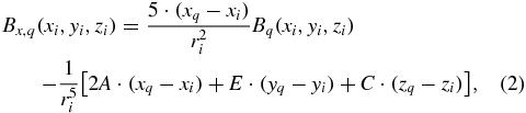
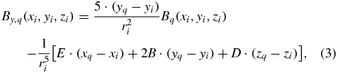
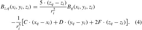
where  , l = cos I0cos A'0, m = cos I0sin A'0, n = sin I0, L = cos Icos A' M = cos Isin A' N = sin I' A = 2 · l · L − n · N − m · M, B = 2 · m · M − l · L − n · N, C = 3 · (l · N + n · L), D = 3 · (m · N + n · M), E = 3 · (l · M + m · L), and F = 2 · n · N − m · M − l · L.
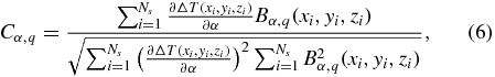
The correlation coefficient between the observed magnetic total field α gradient and the theoretical magnetic total field α gradient caused by the dipole is defined as
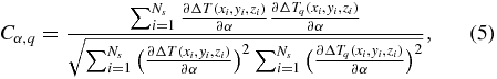
where  is the observed magnetic total field α gradient at the station (xi, yi, zi), and Ns is the total number of the observed stations.
Assuming Mq > 0, then substituting equation (1) into equation (5), gives
According to the Cauchy inequality, the correlation coefficient Cα, q in equation (6) satisfies the condition −1 ⩽ Cα, q ⩽ +1.
The value of Cα, q reflects the cross correlation degree between the observed magnetic total field α gradient and the theoretical magnetic total field α gradient due to the dipole. It implies the probability of finding a magnetic dipole with a total magnetized inclination I and declination A' at point q responsible for the observed α gradient. The lower the absolute value of Cα, q, the lower the probability of the occurrence of a magnetic dipole at point q, while the higher the value of positive Cα, q, a higher probability of the occurrence of a magnetic dipole with a total magnetized inclination I and declination A'. The higher the value of a negative Cα, q, the higher the probability of the occurrence of a magnetic dipole but with the total magnetized inclination and declination different from I and A', respectively.
The approach is called correlation imaging because it derives the subsurface equivalent magnetic dipole distribution in a probability sense by calculating the cross correlation between the observed magnetic total field α gradient and the theoretical magnetic total field α gradient due to the magnetic dipole.
To apply the correlation imaging procedure for the observed magnetic total field α gradient, we first divided the subsurface space into a 2D or 3D regular grid. Then by using equations (6) and (2)–(4), we calculate the correlation coefficient of each node of the 2D or 3D regular grid from the top to bottom, in turn. This yields a correlation coefficient dataset. By visualizing the dataset in 2D or 3D form, we can describe the equivalent magnetic dipole distribution according to the correlation coefficients.
Global correlation coefficient
Different-directional magnetic gradients emphasize structures in particular orientations (Schmidt and Clark 2006). Therefore, to provide a global interpretation of the most likely distribution of magnetic sources, we define a global correlation coefficient function by integrating the three results of the correlation imaging of magnetic total field gradients.
The global correlation coefficient function mainly considers the role of the correlation imaging of the magnetic z-gradient, but also considers the role of the x-gradient and y-gradient. The function takes the maximum of the three correlation coefficients of x, y, and z-gradients when the correlation coefficient of the z-gradient is positive, while it is set to zero when the correlation coefficient of the z-gradient is not positive, because we are mainly interested in the probability of the occurrence of a magnetic dipole with a given total magnetized inclination I and declination A'. Hence, the global correlation imaging function is defined as

The global correlation coefficient Cg, q has no actual physical meaning, because it is obtained by means of a particular composition of the correlation coefficient functions of the three gradients Cα, q(α = x, y, or z). It can be used to comprehensively describe the probability of the occurrence of a magnetic dipole at point q. The value of Cg, q satisfies the condition 0 ⩽ Cg, q ⩽ 1. The closer the value of Cg, q is to 1, the higher the probability of the occurrence of a magnetic dipole with a total magnetized inclination I and declination A' at point q in a global sense.
Data experiments
Test on the synthetic magnetic data
The test model consists of six rectangular prisms with various sizes (see figure 1), among which the bigger prisms A1, A2 and A3 are at deeper depths and the smaller prisms B1, B2 and B3 are in the shallow subsurface. Prisms A1 and B3 have no obvious strike, while prisms A3 and B1 are eastward striking and prisms A2 and B2 are northward striking. The geometric parameters of each prism are listed in table 1. The total magnetization of each prism is 1 A m−1, and the total magnetized inclination and declination are, respectively, 80° and −50°. The inclination and declination of the geomagnetic field are, respectively, 45° and −5°. We did the forward modelling of the model for the magnetic total field x, y and z-gradients on a topographic surface (figure 2(a)). The observed geometry is a 201 × 201 regular grid with a grid spacing of 0.04 km along both easting and northing. Then the three synthetic magnetic total field gradients were all contaminated by Gaussian noise (figures 2(b)–(d)).
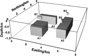
Figure 1. 3D visualization of the synthetic model.
Download figure:
Standard image
Figure 2. (a) The observed surface topography, in which the black solid lines show the locations of profiles A–A', B–B', C–C' and D–D'. (b)–(d) are respectively the x-gradient, y-gradient and z-gradient of the magnetic total field anomaly of the model. All of the gradients were contaminated by Gaussian noise.
Download figure:
Standard imageTable 1. The geometric parameters of the synthetic rectangular prisms (unit: km).
| Prism ID | Length along easting | Length along northing | Thickness | x of the centre | y of the centre | z of the centre |
|---|---|---|---|---|---|---|
| A1 | 1.6 | 2 | 0.6 | 2.7 | 2.5 | 0.9 |
| A2 | 1.2 | 4 | 0.6 | 5.8 | 4 | 0.9 |
| A3 | 2.6 | 0.6 | 0.6 | 2.7 | 5.6 | 0.9 |
| B1 | 0.64 | 0.16 | 0.16 | 2.52 | 3 | 0.24 |
| B2 | 0.16 | 0.4 | 0.16 | 5.6 | 3 | 0.24 |
| B3 | 0.24 | 0.24 | 0.16 | 5.6 | 5.6 | 0.24 |
Then we tested the correlation imaging approach on the synthetic magnetic total field x-, y- and z-gradients, respectively, with a depth extent of −1.2 km∼0 km and a depth step of 0.04 km. Here the total magnetized inclination 80° and declination −50° of magnetic dipole are used in equations (2)–(4).
Figure 3 shows the images of the correlation coefficients derived from the correlation imaging of the synthetic magnetic total field x-gradient along profiles A–A', B–B', C–C' and D–D' (shown with black lines in figure 2(a)). The outline of the true prisms was drawn by black lines in each image section. Figure 4 displays those of the synthetic y-gradient, and figure 5 displays those of the synthetic z-gradient. The high positive correlation coefficients shown by the bright colour portions in figures 3–5 indicate a high probability of the occurrence of a magnetic dipole with the total magnetized inclination 80° and declination −50°.

Figure 3. The equivalent magnetic dipole distribution (image sections) derived from the correlation imaging of the x-gradient (graph sections) along profiles A–A' (a), B–B' (b), C–C' (c) and D–D' (d). Black lines in the image sections show the outline of the true prisms.
Download figure:
Standard image
Figure 4. The equivalent magnetic dipole distribution (image sections) derived from the correlation imaging of the y-gradient (graph sections) along profiles A–A' (a), B–B' (b), C–C' (c) and D–D' (d). Black lines in the image sections show the outline of the true prisms.
Download figure:
Standard image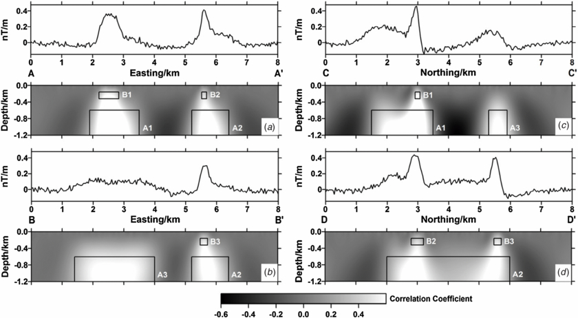
Figure 5. The equivalent magnetic dipole distribution (image sections) derived from the correlation imaging of the z-gradient (graph sections) along profiles A–A' (a), B–B' (b), C–C' (c) and D–D' (d). Black lines in the image sections show the outline of the true prisms.
Download figure:
Standard imageFrom figures 3–5, we can see that all of the correlation imaging of the three gradients produces high positive correlation coefficients inside the outline of prisms A1 and B3, which have an approximate equi-axed shape. This means that they all can reveal causative sources with an approximate equi-axed shape. Both the correlation imaging of the x-gradient and the z-gradient produce high positive correlation coefficients inside the outline of prisms A2 and B2 (see figures 3 and 5), which have a northward strike. This indicates that they both can reveal causative sources with a northward strike. Both the correlation imaging of the y-gradient and the z-gradient produce high positive correlation coefficients inside the outline of prisms A3 and B1 (see figures 4 and 5), which have an eastward strike. This implies that they both can reveal causative sources with an eastward strike. Therefore, the correlation imaging of different-directional magnetic gradients can reveal magnetic sources with different strike. We used global correlation imaging to obtain a global interpretation of the most likely distribution of magnetic sources.
We then calculated the global correlation coefficient function of the three gradients at each node in the subsurface regular grid by using equation (7). Figures 6(a)–(d) show the images of the global correlation coefficients along profiles A–A', B–B', C–C' and D–D', respectively. High positive correlation coefficients occur clearly inside the outline of both the deep prisms A1–A3 and the shallow prisms B1–B3 in figure 6, which indicates that the global correlation coefficient function can reveal causative sources with almost all kinds of strike.

Figure 6. The equivalent magnetic dipole distribution derived from the global correlation imaging of the three gradients along profiles A–A' (a), B–B' (b), C–C' (c) and D–D' (d). Black lines in the image sections show the outline of the true prisms.
Download figure:
Standard imageTest on the real magnetic data
The real magnetic total field anomaly data (figure 7) is taken from a metallic deposit area in the middle-lower reaches of the Yangtze River in China. The data were observed on a fairly flat surface with an average elevation of 15 m, and was gridded on a 132 × 101 regular grid with a grid spacing of 0.05 km along both easting and northing. The inclination and declination of the geomagnetic field are 46.65° and −4.4°, respectively. None of the magnetic total field gradients were observed directly.

Figure 7. The real magnetic total field anomaly from a metallic deposit area in China. White line shows the location of profile A–A'.
Download figure:
Standard imageThe deposit is located in the effusive rock basin formed during the faults and magma activities in the late Yanshan period (Mesozoic age). The metallic ore includes magnetite, specularite and chalcopyrite with strong magnetism, and mainly occurs in faults or fracture zones, intrusive contact zones and depression-uplift structures of the effusive rock basin. The background terrane is effusive rock with medium magnetism and sedimentary rock with almost no magnetism. The magnetic source distribution in the subsurface remains unknown due to no existing borehole and little a priori geological information for this area. Here, we tried to use the correlation imaging approach to obtain a rough imaging of the subsurface.
We firstly calculated the x-, y- and z-gradients of the real magnetic total field anomaly by the conventional Fourier transformation method. Then we tested the correlation imaging approach, on the calculated x-, y- and z-gradients, respectively, with a depth extent of −1.5–0 km and a depth step of 0.05 km. In this case, assuming that the effects of remnant magnetization and demagnetization can be neglected, the inclination and declination of total magnetization of the magnetic dipole used in equations (2)–(4) were the same as those of the geomagnetic field. Then we calculated the global correlation coefficient function of the three gradients at each node of the subsurface regular grid according to equation (7). Figures 8(a)–(c) show the images of the correlation coefficients derived from the correlation imaging of the x-, y- and z-gradients, respectively, along profile A–A' (white line in figure 7), and figure 8(d) displays the image of the global correlation coefficients.

Figure 8. The equivalent magnetic dipole distribution derived from the correlation imaging of the x-gradient (a), y-gradient (b) and z-gradient (c) along profile A–A', and that from the global correlation imaging of the three gradients (d). The black downward arrow on the top right-hand side of each image section shows the location of the borehole. The top of the figure shows the real magnetic total field anomaly along profile A–A'.
Download figure:
Standard imageHigh positive values of correlation coefficients alternate with low positive or negative values above a depth of −0.5 km in each image section of figure 8. This indicates a laterally heterogeneous magnetism distribution in the shallow depths. A large zone of high positive correlation coefficients occurs at a distance range of 0.6–1.4 km and below a depth of −0.5 km as shown in figures 8(a)–(c), which implies a high probability of the occurrence of a magnetic source with an approximate equi-axed shape. Another large zone of high positive correlation coefficients appears at a distance range of 4.7–5.3 km and below a depth of −0.5 km, which is shown in figures 8(a) and (c) but disappears in figure 8(b). This implies a high probability of the occurrence of a magnetic source with an approximately northward strike. These two large zones of magnetic source distribution are delineated more directly and clearly in the global correlation coefficients image section (figure 8(d)).
Based on the above results and the preliminary geological evaluation, one borehole was drilled at a distance of 5.1 km in profile A–A' (the black downward arrow in each image section of figure 8). The borehole was drilled to a depth of −1.3 km. The rock core is andesite above a depth of −1.17 km while it is syenite below this depth. The metallic ores of specularite, magnetite and chalcopyrite were found among the crack and fracture zones of the andesite terrane. Specularite of 2.5–4 m thickness was found at depths of −0.243, −0.356 and −0.710 km, respectively. Magnetite of 2–3 m thickness was found at depths of −0.818 and −0.871 km, respectively. Chalcopyrite of 3–9 m thickness was found at depths of −0.340, −0.954, −0.979 and −1.101 km, respectively.
Conclusions
We have introduced a correlation imaging approach for the magnetic total field x-, y- and z-gradients for producing an equivalent magnetic source distribution of the subsurface in a probability sense. We have also defined the global correlation coefficient function of the gradients to comprehensively describe the probability of the occurrence of magnetic dipoles in the subsurface. Tests on synthetic magnetic data and actual magnetic data show that the correlation imaging of the x-gradient reveals magnetic sources with a northward strike and the correlation imaging of the y-gradient reveals magnetic sources with an eastward strike. The correlation imaging of the z-gradient can disclose magnetic sources with any kind of directional strike. The tests also demonstrate that the global correlation coefficients delineate a more direct and comprehensive magnetic source distribution in the subsurface. The global correlation imaging approach can be used to provide a global evaluation of the most likely distribution of magnetic sources ahead of detailed and precise interpretation, especially when no or little a priori information is available.
Acknowledgments
We thank two anonymous reviewers for their helpful comments and valuable suggestions. This work was supported by the National Natural Science Foundation of China (40904033), the Fundamental Research Funds for the Central Universities and the SinoProbe projects (201011039).