

Abstract
The seismic modulation model analyzes a seismogram from the low and high-frequency information, which is different from the traditional convolution model. In the modulation model, a seismogram is regarded as a modulated signal and its envelope is the amplitude-modulation component containing the low-frequency information. On this foundation, the envelope of seismograms can be used to recover a very smooth background structure. However, amplitude demodulation methods can only obtain the absolute value of the envelope, which cannot reflect the polarity changes of the amplitude information in seismograms. To solve this problem, we consider the low-frequency modulation from both the amplitude and polarity points of view. We extract a modulator signal with smoothed apparent polarity, which contains the amplitude and polarity information in seismograms. The new approach can broaden the modulation model theory for seismic signals. Good results from examples for application to envelope inversion demonstrate the good performance and potential of the proposed method.
Export citation and abstract BibTeX RIS
Introduction
Historically, most signal analysis is based on linear transforms, which are additive decompositions. It assumes that a signal can be represented by a superposition of independent components. This is the principle of linear superposition, such as in the traditional linear data transforms, e.g., Fourier transform, Hilbert transform, or other transforms using basis and frames.
The modulation–demodulation transform is a nonlinear multiplicative decomposition which can reveal the structure of the process, such as the trends, slow evolution and variation, secular force for dynamics, etc. On the other hand, linear decompositions, such as the Fourier transform, assume each component of the process as independent from the other components. In the time domain, the modulated signal equals to the product of the modulation signal and the carrier signal. When a Fourier transform is performed to a modulated signal, the Fourier spectrum of the modulated signal is convolved with the Fourier spectrum of the carrier signal. It means that the low-frequency band of the modulation signal moves towards the high-frequency ends of the carrier frequency, so one will have a frequency shift to high frequencies, and a frequency split of the carrier frequency. In the end, the low-frequency modulation signal cannot be found by using the Fourier decomposition method. The linear decomposition and processing can only change the relative magnitude of the spectral components of the signal without generating new frequency components. So the linear decomposition cannot recover the missing low-frequency information in the signal. That is why waveform inversion based on a linear signal model cannot see the ultra-low-frequency information that is lower than the lowest frequency contained in the source wavelet. From the modulation model, the ultra-low-frequency information is in the envelope which can be extracted nonlinearly by a demodulation operator.
Wu et al (2014) proposed an envelope inversion (EI) method to extract the ultra-low-frequency information contained in seismograms, and considered the signal model for seismograms as a seismic modulation–convolution model. This new signal model can fully represent the low-frequency and high-frequency information. Historically, the observed seismic records are commonly modeled as the convolution of the source wavelet and the Earth's reflectivity series. The traditional convolution signal model (Robinson et al 1986) is a linear model suitable for seismic imaging. However, seismograms contain other information that the convolution model does not include. The modulation signal model provides a novel perspective for seismic exploration (Luo and Wu 2015, Hu et al 2017, Wang and Wu et al 2017, Wang and Yuan et al 2017, Wu and Chen 2017a, 2017b).
The modulation modeling technique has been successfully applied to some research fields, such as speech signal analysis (Potamianos and Maragos 1999) and image processing (Havlicek et al 1996), and thus propelled the development of many demodulation methods (Loughlin and Tacer 1996, Turner and Sahani 2011, Xu et al 2014). However, most amplitude demodulation methods can only obtain the positive envelope, which cannot reflect the polarity changes in seismograms. Polarity plays an important role in the seismic instantaneous attributes, and many researches have been done on its definition and criterion (Taner et al 1979, Robertson and Nogami 1984, White 1991, Brown et al 2002, Sheriff 2012, Wang et al 2016). Polarity can be defined as the sign of reflection coefficient that indicates an increase or decrease in the interfacial wave impedance. So the EI without polarity information can not characterize the situation of wave impedance reduction. Xu et al (2014) proposed a signed demodulation method for amplitude and frequency modulation signal. But this signed demodulation theory is mainly applicable to the sine and cosine modulation signal, not suitable for seismograms. Taner et al (1979) proposed the concept of apparent polarity, which can represent the polarity information of seismogram. Inspired by the research above, we propose including polarity information in the demodulation of seismograms and in the application of EI.
The seismic modulation model
Using the modulation signal model, Wu et al (2014) proposed that the reflection seismogram  formed by backscattered waves with geophone
  and source
  is modeled as


where  serves as the carrier formed by the convolution of the source wavelet
  and the reflection coefficient function
 is a Dirac delta function, and
  is a smoothly varying Green's function pair (background propagator) which serves as the modulator and only modifies the traveltimes and amplitudes of the reflection events.
In the modulation signal model,  still contains useful low-frequency information of the medium velocity structure. In order to model the information contained in the seismogram, we decompose the seismogram
  into two multiplicative components: a low-frequency component
  and a high-frequency component
  that is

The low-frequency component  of the seismogram can be demodulated as Hilbert envelope, that is
where ![$H[\cdot ]$](https://content.cld.iop.org/journals/1742-2140/15/5/2278/revision2/jgeaac54dieqn14.gif) denotes Hilbert transform operator, and
denotes Hilbert transform operator, and ![$E[\cdot ]$](https://content.cld.iop.org/journals/1742-2140/15/5/2278/revision2/jgeaac54dieqn15.gif) is envelope operator. In the demodulation process, the Green's function
is envelope operator. In the demodulation process, the Green's function  is pulled out of the Hilbert transform because it is a smooth function satisfying the Bedrosian–Brown's condition for Hilbert transform (Bedrosian 1962, Brown 1986). However, the low-frequency component in equation (4) contains only positive amplitude without polarity information.
In fact, the multiplicative decomposition 3 is non-unique and therefore has many possible solutions. We reconsider a demodulation method to obtain a low-frequency component with polarity information.
We assume that the low-frequency component contains two parts: a positive Hilbert envelope and a smooth polarity curve. Then the low-frequency component  of seismogram can be reformulated as

where  represents the smooth polarity curve. In this expression, the envelope
  determines the magnitude of the low-frequency component, and
  is a smoothing curve with polarity. The low-frequency component
  contains the amplitude and polarity information of the seismogram, representing the information on the smoothed medium velocity structure. When the seismogram contains noise, its Hilbert envelope will have the high-frequency components caused by noise, and the
  curve will also be affected. Correspondingly, there are high-frequency components of noise in the
  In this case,
  should be the data after low-pass filtering to reduce the influence of noise.
Smoothed apparent polarity
The apparent polarity is proposed by Taner et al (1979), defined as the sign of signal when Hilbert envelope has a local maximum. Assuming a single reflection, a zero-phase wavelet and no phase reverse, a positive or negative sign can be used to refer to positive or negative reflection coefficients. However, that is the ideal situation. Generally, most reflection events consist of multiple reflectors. The interference between the reflectors may cause the location of the local maximum of the envelope to be inconsistent with the position of the reflection coefficient, so that there is a lack of clear correlation between the sign and the reflection coefficient. Hence, the sign is regarded as apparent polarity, showing a rough polarity of the seismogram.
From the definition, the apparent polarity has a value only at the local maximum of the envelope. If the apparent polarity is considered as a portion of the low-frequency component, we need to generate a smooth apparent polarity curve by using these points. In this paper, we consider a zero-phase Ricker wavelet as the source wavelet, and get a smoothed apparent polarity (SAP) by interpolation to represent the low-frequency polarity information of the seismogram.
Given a signal  with
with  sample points, if it contains noise, a low-pass filter is applied to the signal first. Then its envelope with smoothed apparent polarity (E-SAP) can be obtained as follows with the outline in figure 1:
- (1)Take the Hilbert transform of the signal
 and obtain the envelope Identify all local maxima of denoted as ( represents the coordinate location of local maxima);
 - (2)Get the apparent polarity of all local maxima points (if ), and set the apparent polarity at beginning and end to zero, that is,
- (3)Add an adjacent point to both sides of the local maxima that is, and Connect all the apparent polarity points by a cubic spline line as the smoothed apparent polarity
- (4)The E-SAP of signal can be obtained by


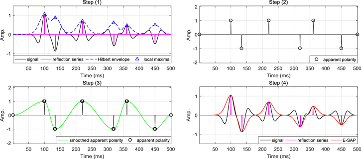
Figure 1. The outline of E-SAP. The black line represents the signal; the pink line represents the reflection series; the blue dotted line represents the Hilbert envelope of signal; and the blue triangles are the local maxima of the Hilbert envelope; the black circles are apparent polarity points at the local maxima of the Hilbert envelope; the green line represents the smoothed apparent polarity obtained by interpolation; and the red line represents the E-SAP result.
Download figure:
Standard image High-resolution imageIn step (2), we make  at
at  to prevent the situation that apparent polarity equals 0 at the local maxima due to interferences. In addition, setting the apparent polarity at the beginning and end to zero is to ensure that the interpolation curve does not have large derivations at the beginning and end. In step (3), adding adjacent points is to stabilize the interpolation curve, which can be proved by figure 2. It is evident that adding adjacent points makes the interpolation curve more stable and prevents excessive amplitude in the SAP result. The interpolation curve without adding adjacent points (figure 2(c)) is easy to deflect, so that the E-SAP result (figure 2(d)) would be badly affected.
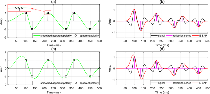
Figure 2. SAP and E-SAP result (a)–(b) with adding adjacent points and (c)–(d) without adding adjacent points.
Download figure:
Standard image High-resolution imageIn addition, the performance of E-SAP depends on the local maxima of Hilbert envelope. As shown in figure 3, we give the synthetic seismogram of a wedge model that is generated by a wavelet convolved with two reflections of equal amplitude and opposite polarity, and the layer thickness between two reflections is gradually decreasing. The layer thickness has an influence on the detection of the local maxima of the envelope. When the local maxima of the upper and lower boundaries can be separated, the E-SAP can characterize the polarity reversal. However, as the layer thickness decreases, the interference between the two reflections becomes stronger, so that the two local maxima are confused. In figure 3, for a signal with layer thickness less than 26 ms, the E-SAP gives the same result as the Hilbert envelope without polarity reversal. Therefore, if all the local maxima of envelope are not detected due to the presence of thin beds or other interferences, the E-SAP can not reflect the polarity reversal between layers. In this case, the E-SAP result is almost identical to the Hilbert envelope. So, even if the local maxima of the envelope is biased, the SAP is a slow-varying curve of polarity without amplitude gain, which does not cause serious damage to the E-SAP result.
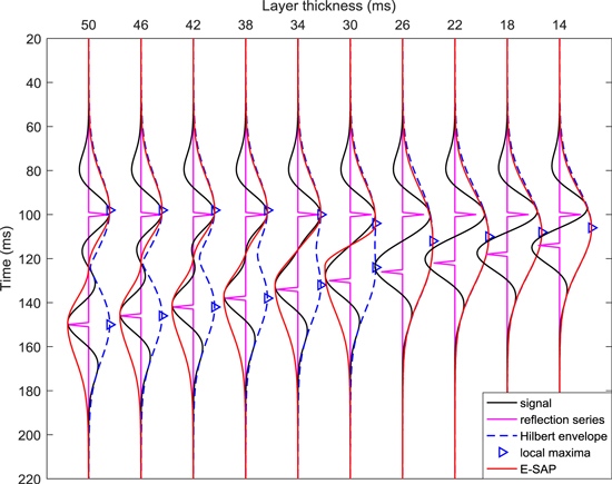
Figure 3. Wedge model that a wavelet convolved with two spikes of equal amplitude and opposite polarity.
Download figure:
Standard image High-resolution imageExperiments and analysis
Single-trace
A single-trace without thin layer is generated by a series of reflection coefficients convolved with a 20 Hz Ricker wavelet as shown in figure 4. The ten reflectors are located at 140, 200, 320, 360, 460, 520, 666, 700, 750 and 900 ms. The Hilbert envelope (figure 4(a)) is always positive, which cannot reflect the polarity changes of the amplitude. All the local maxima of envelope around the reflection series are identified. So the E-SAP result in figure 4(c) shows a rough smooth fitting curve of the reflection series, which contains the polarity information of trace. Figures 4(b) and (d) give the frequency spectrum distribution of trace, Hilbert envelope and E-SAP. We can see that the Hilbert envelope and E-SAP contains the low frequencies below the frequency range of trace. Figure 5 shows another single-trace with a thin bed produced by multiple reflection coefficients convolved with a 20 Hz Ricker wavelet. The ten reflectors are located at 140, 200, 320, 335, 460, 520, 666, 700, 750 and 900 ms. The wavelength of the Ricker wavelet can be estimated by  where
where  is the peak frequency (Kallweit and Wood 1982). The thickness of the thin bed at 320–335 ms is below the quarter wavelength. The Hilbert envelope (figure 5(a)) at the thin bed (dotted ellipse) only has one local maxima so that the E-SAP (figure 5(c)) does not reverse the polarity. However, the E-SAP result gives the polarity changes at other locations (dotted box). The corresponding spectral range is still below the frequency band of trace.

Figure 4. A synthetic trace response of ten reflectors convolved with a 20 Hz Ricker wavelet. Hilbert envelope in the time domain (a) and frequency domain (b); E-SAP in the time domain (c) and frequency domain (d).
Download figure:
Standard image High-resolution image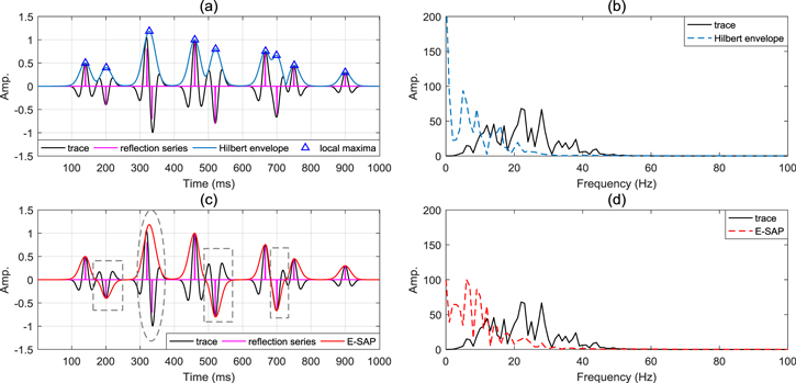
Figure 5. A synthetic trace with a thin bed response of ten reflectors convolved with a 20 Hz Ricker wavelet. Hilbert envelope in the time domain (a) and frequency domain (b); E-SAP in the time domain (c) and frequency domain (d).
Download figure:
Standard image High-resolution imageThe proposed method is also a test on a noisy single-trace as shown in figure 6. The noisy single-trace is generated by adding white Gaussian noise into the single-trace in figure 5, giving a signal-to-noise ratio of 5 dB. The Hilbert envelope (figure 6(a)) removes the high-frequency components of noise, and the E-SAP result (figure 6(c)) still give the polarity changes at 200, 520 and 700 ms (dotted box). And their frequency spectral removes the high-frequency range of noisy trace.

Figure 6. A synthetic noisy trace with a thin bed response of ten reflectors convolved with a 20 Hz Ricker wavelet. The noisy trace is added with white Gaussian noise, giving a signal-to-noise ratio of 5 dB. Hilbert envelope in the time domain (a) and frequency domain (b); E-SAP in the time domain (c) and frequency domain (d).
Download figure:
Standard image High-resolution imageApplication in EI
The full-waveform inversion (FWI) requires a good initial model and performs poorly when the source wavelet misses the low-frequency information (Virieux and Operto 2009). To overcome these deficiencies, the EI and its related methods are developed. The misfit function of conventional EI is defined as
where  is the envelope of a synthetic wavefield, and
  is the envelope of an observed waveform data. The summation is over all the sources
  and receviers
  We use the new direct Envelope Fréchet derivative
  to get the sensitivity operator for EI (Wu and Chen 2017a, 2017b) and the gradient operator for EI is

where summation of  is over the source, receiver and time,
  is the velocity model parameter,
  is virtual source operator,
  is the envelope Green's operator representing the forward propagation process, and
  is the adjoint operator of
  representing the reverse-time propagation of the envelope residual
  (For detailed formulation see Chen et al 2017, Wu and Chen 2017b and Chen et al 2018.) In the EI, the Hilbert envelope is defined as envelope operator. In this paper, the E-SAP is used as the new envelope operator instead of the Hilbert envelope. The EI result obtained by E-SAP is denoted as SAP-EI. We also compare the performance of the Hilbert envelope and E-SAP in the combined EI + FWI inversion (Wu et al 2014). In the combined inversion, the FWI result is obtained by using the smooth background from EI as the initial model. In addition, the source wavelet used in the inversion is a low-cut Ricker wavelet (cut from 4 Hz below).
We use two models to verify the effectiveness of the E-SAP method in the EI. Figure 7(a) shows the test model which has three low-speed horizontal layers (T1, T3, T5), three high-speed horizontal layers (T2, T4, T6), and a high-speed block B. The high-speed (red) is 5 km s−1 and low-speed (blue) is 3 km s−1. There are 80 shots distributed along the model surface at intervals of 20 m and 240 receivers with intervals of 20 m for each shot. And the initial model is a linear gradient model given in figure 7(b). The source wavelet is a Ricker wavelet with the dominant frequency 9 Hz, and the frequency component below 4 Hz is removed.
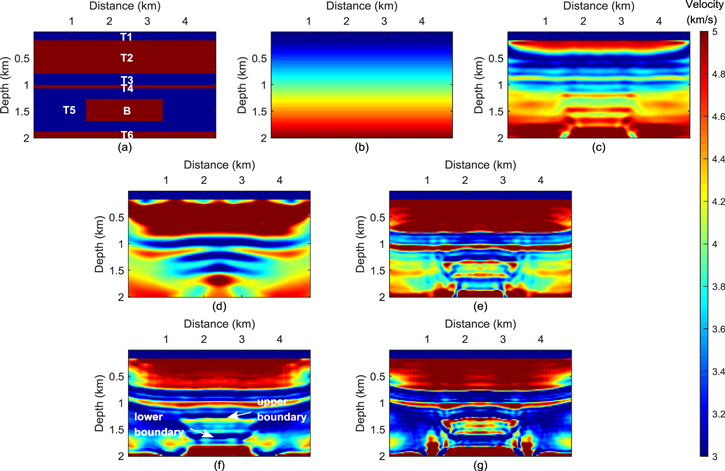
Figure 7. Test model and inversion results using the low-cut source. (a) A velocity model with six horizontal layers (three low-speed layers (T1, T3, T5) and three high-speed layers (T2, T4, T6)) and a high-speed block B; (b) linear gradient initial model; (c) FWI inversion result; (d) Hilbert envelope EI inversion result; (e) Hilbert envelope EI + FWI inversion result; (f) SAP-EI inversion result; (g) SAP-EI + FWI inversion result.
Download figure:
Standard image High-resolution imageFor comparison, in figure 7(c), we show the FWI inversion result directly using the linear initial model. The traditional FWI result has large deviations from the S2 layer, which fails to give the whole structure of the model. The inversion results by Hilbert Envelope EI and SAP-EI are given in figures 7(d) and (f), respectively. The Hilbert Envelope EI fills the velocity well in the T2 layer, but performs poorly for the structure below T2 layer. A better inversion result of the structure is obtained by SAP-EI. The SAP-EI result recovers the six horizontal layers, but deviates from 1.3 km due to the influence of high-speed block B. Although SAP-EI does not reconstruct the high-speed block B well, it clearly outlines the upper and lower boundaries. In the inversion result of SAP-EI, the velocity filling of T2 layer is not as good as EI, but the boundaries of layers are better characterized. In addition, we also give the combined EI plus FWI inversion results. Figures 7(e) and (g) show the final results of combined EI + FWI inversion using the recovered smooth background by EI. It can be seen that there are significant improvements in the inversion results by combined inversion EI + FWI. The EI + FWI using Hilbert envelope performs better than the EI alone, but it still fail to obtain an accurate estimate of the target model, especially in the low-speed layer T5. The SAP-EI + FWI inversion result is closer to the true velocity model.
We select one trace from the 60th shot data generated using the model with the low-cut source wavelet as shown in figure 8. In figure 8(a), the Hilbert envelope produces a positive smooth envelope for the trace, while the SAP produces a smooth curve with positive and negative polarity. For convenience of display and comparison, the amplitude unit of the frequency spectrum is converted to dB. In figure 8(b), the original seismic trace lacks the low-frequency component below 4 Hz, while the Hilbert envelope and E-SAP contain rich low-frequency information.
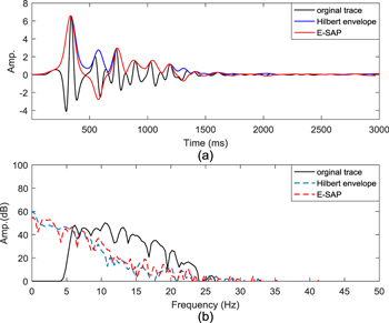
Figure 8. One trace selected from the 60th shot data generated from the model and its envelopes in the time domain (a) and frequency domain (b).
Download figure:
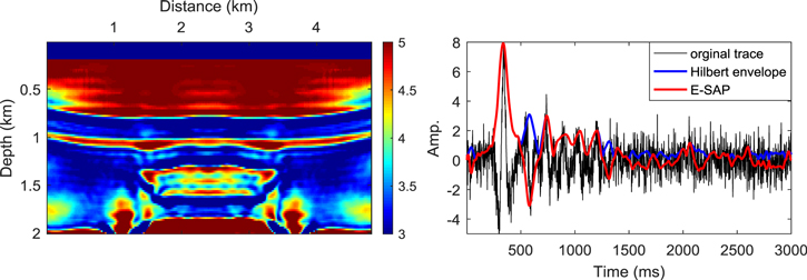
Standard image High-resolution imageConsidering the effect of noise, we add white Gaussian noise with signal-to-noise ratio of 5 dB into the shot data to test the anti-noise capability of the proposed method. We pre-filter the shot data with a low-pass filter and then obtain the SAP-EI + FWI inversion result shown in figure 9 (left), which still give an accurate estimate of the true velocity model under the noise interference. Figure 9 (right) represents the Hilbert envelope and E-SAP result of one trace from the 60th noisy shot data. These results are obtained after low-pass filtering on the noisy trace. Similar to the no-noise condition, the Hilbert envelope gives a positive smooth envelope, and the E-SAP gives a smooth curve with positive and negative polarity. The robustness of E-SAP is verified by the noisy data testing. The experiments indicate that the E-SAP can obtain the low-frequency information with polarity of seismogram, and perform well even in a noisy situation.
Figure 9. The SAP-EI + FWI inversion result in the case of white Gaussian noise with signal-to-noise ratio of 1 dB (left), and its one trace selected from the 60th noisy shot data and its envelopes in the time domain (right).
Download figure:
Standard image High-resolution image
Conclustion
The modulation signal model can provide low-frequency and high-frequency information of a seismogram, especially for the ultra-low-frequency information which is lost in the convolution model. A reasonable demodulation method is required for extracting the low-frequency component. In the seismic modulation model, the low-frequency component is usually extracted as a positive envelope by most demodulation methods, losing the polarity information of the seismogram. Inclusion of polarity information is important to characterize the reflected energy of different interfaces. On this basis, we proposed an envelope with smoothed apparent polarity (E-SAP) as a new demodulation method. The E-SAP contains the smooth amplitude and polarity information of the seismograms. In addition, we applied the E-SAP to the EI as new envelope operator instead of Hilbert envelope. Compared with convention EI, the EI using E-SAP can better reconstruct the velocity structure and characterize the boundary. The numerical examples demonstrated the effectiveness of the proposed method and its good performance in the EI and combined EI + FWI.
Acknowledgments
This work is supported by the WTOPI Research Consortium at University of California, Santa Cruz, USA. Y Wang acknowledges the financial support from China Scholarship Council and the National Natural Science Foundation of China (Grant Nos. 61571096, 41274127 and 40874066).