
Abstract
With the development of seismic exploration technology, the wave equations used to model the characteristics of wave propagation are becoming increasingly complex. Generally, more than one physical parameter is included in these wave equations, and merely inverting one parameter from these equations cannot help to accurately understand the subsurface structure. To gain further insight into the structure or oil- and gas-reservoir characteristics of the subsurface, multi-parameter inversion is essential. In this study, density, velocity, and viscosity coefficient are jointly reconstructed from the Stokes equation by frequency-domain full waveform inversion based on zero-offset VSP data. The inverse problem is transformed to find the optimal solution to an optimization problem, and the steepest-descent method is used. The sensitivities of the parameters to the misfit function are analysed. Two inversion strategies, namely, the one-by-one parameter inversion and joint inversion strategies, are tried and compared. The joint inversion strategy is proved to be better and thus used in subsequent analyses. In the numerical tests, we compare different frequency-selection strategies and determine the influences of initial models and number of frequencies to the rebuilt models. Numerical tests show that multi-parameter inversion by frequency-domain FWI is feasible and reliable.
Export citation and abstract BibTeX RIS
1. Introduction
With the development of seismic exploration techniques, wave equations can realistically model wave propagation under the subsurface. However, the equations are becoming more complex and including more parameters. Obtaining multi-parameters by inversion can help to accurately illustrate the subsurface structure.
In recent years, the application of full waveform inversion (FWI) for imaging subsurface parameters has received increased interest. Numerous studies have been conducted from different aspects as follows: to reduce the computation cost in each iteration, phase encoding approaches are used in FWI (Krebs et al 2009, Tao and Sen 2013); to improve the inversion accuracy, optimization methods used in FWI have been developed from the steepest-descent method (Gauthier et al 1986) to the Gauss–Newton method (Kang et al 2012, Hu et al 2009) and to the full Newton method (M'etivier et al 2012, Anagaw and Sacchi 2012); and so on. In these studies, the parameter velocity is the most commonly inverted parameter (Anagaw and Sacchi 2012, Gauthier et al 1986, Krebs et al 2009, M'etivier et al 2012, Mora 1988, Pratt and Worthington 1990, Pratt 1990, Ravaut et al 2004, Sourbier et al 2009, Tao and Sen 2013). In these cases, other parameters are set to be perfectly known even though they are unknown in reality. If more parameters apart from the velocity can be obtained, this problem can be avoided. However, multi-parameter inversion is a computationally challenging problem. With an increased number of inverted parameters and stronger uncertainties, the inversion becomes more prone to obtaining local minimum solutions. Moreover, some parameters are coupled and become difficult to invert separately at the same time.
Among the studies on FWI, only a few applications of multi-parameter inversion have been presented. Brossier et al (2009) successfully imaged the Vp and Vs model jointly from the onshore inversions of the synthetic SEG/EAGE overthrust model by frequency-domain FWI. Barros et al (2010) showed that the inversion procedure could accurately reconstruct a single model parameter if all other parameters were perfectly known, and then they composited coupled parameters as one parameter to invert only one parameter. Malinowski et al (2011) reconstructed Vp and Q jointly and applied the method to real field data. Jeong et al (2012) proposed a two-stage elastic FWI strategy to recover density as well as Vp and Vs jointly. Kang et al (2012) performed FWI to obtain Vp and Vs from isotropic fluid–solid media. Indeed, multi-parameter inversion is a challenging problem that still requires extensive efforts.
Our study presents a multi-parameter inversion of density, velocity, and viscosity coefficient jointly from the Stokes equation by frequency-domain FWI from zero-offset VSP data. The Stokes equation was first proposed by Stokes (1845) to describe the attenuation phenomenon of acoustic wave propagation in an air medium. The equation considers energy loss caused by viscous friction, and has been successfully applied to describe the propagation and attenuation of acoustic waves in an air medium. To solve the problem of the considerable differences between the sinusoidal seismic records obtained from field exploration and the modelled pulse seismic records from the classic elastic theory, Ricker (1977) introduced the Stokes equation into the wave propagation on Earth. Ricker (1977) found that high-frequency components are filtered by the Earth filter and the residual low frequency parts suffer from absorption from the viscous friction, in agreement with the experimental results. The results show that the Stokes equation should be applied to the seismic phenomenon instead of the classic wave equation. For the attenuation effect in seismic propagation, one way is to introduce the complex velocity by the quality factor Q (Brossier 2011, Hicks and Pratt 2001, Malinowski et al 2011, Ravaut et al 2004, Sourbier et al 2009, Takougang and Calvert 2012), and Q is commonly obtained in the frequency domain. However, in the Stokes equation, the attenuation effect depends on the viscosity coefficient that can be solved either in the time or frequency domains. Liu et al (2000) gave an approximate formula to illustrate the relationship between Q and viscosity coefficient, which showed that Q was inversely proportional to the attenuation while viscosity coefficient was proportional to the attenuation. In essence, the two ways of attenuation are equivalent to each other.
Ricker (1977) also pointed out that in all three styles of solid, liquid, and air media, the Stokes equation can be used for minor perturbation to describe propagation in these media. However, the Stokes equation is rarely applied apart from acoustic wave attenuation in an air medium. The reason is that the Stokes equation is a three-order partial differential equation (PDE) that is difficult to be solved compared with second-order PDEs (Ricker 1977). Ricker (1977) studied the plane-wave solution of the Stokes equation in a seismic field as well as the relation between attenuation and frequencies. Liu et al (2002) pioneered the application of a time-domain finite difference method to this equation to model seismic propagation. For the inverse problems of the Stokes equation, only Liu et al (2006) performed a three-parameter inversion of density, velocity, and viscosity coefficient by a pulse spectrum technique in the mixed time and frequency domains. However, their inverted results are not convergent with the true models. In our study, these parameters are jointly reconstructed by frequency-domain FWI, which can finally provide more information for accurately characterizing the subsurface structures.
We implement FWI in the frequency domain, which presents some distinct advantages with respect to the time-domain FWI (Pratt and Worthington 1990, Pratt 1990, Brossier et al 2009). The gradient of the objective function is computed with the adjoint-state technique (Brossier et al 2009). Inversions of proceeding hierarchically from the low to high frequencies produce a multiscale inversion algorithm. Moreover, inverting a limited number of frequencies can be sufficient to build reliable models.
In the second section, we briefly review the theory of frequency-domain forward modelling and FWI. In the third section, we analyse the sensitivity of the parameters and compare two inversion strategies. In the fourth section, the chosen inversion strategy is applied to reconstruct density, velocity, and viscosity coefficient from synthetic zero-offset VSP data. Three frequency selection strategies are compared to identify the optimal one as well as to determine the influences of initial models and number of frequencies on the inverted models. In the last section, we give the conclusions.
2. Method and algorithm
2.1. Forward problem
For seismic modelling, the Stokes equation can be obtained by adding the absorbing term to the classical inhomogeneous elastic equation (Ricker 1977) in the time domain expressed as
Considering the first-order hyperbolic system with the perfectly matched layer (PML) boundary conditions, we can obtain
where u(z, t) is the time domain wavefield and f is the time domain source function; ρ(z), υ(z), and η(z) are the density, velocity, and viscosity coefficient, respectively; γ(z) is the damping function in the PML boundary conditions; and q(z, t) is the stress.
Then, we transform (2) and (3) into frequency domains by Fourier transformation, and after some calculations we can obtain
where  , ω is the angular frequency, U(z, ω) is the frequency domain wavefield, and Q(z, ω) is the frequency domain stress.
Equations (4) and (5) are discretized by the fourth-order space finite-difference scheme based on the staggered-grid formulation (Levander 1988). The PML method is used for absorbing boundary conditions along the edges of the model. The discretization format leads to solving the linear system

where A is the impedance matrix that depends on the angular frequency and medium properties, F is the source term, and U represents wavefields. Equation (6) is solved by using the LU factorization method.
2.2. Inverse problem
2.2.1. Inverse algorithm
FWI is an optimization problem that can be recast as a linearized least-squares problem that attempts to minimize the misfit between the recorded and modelled wavefields (Tarantola 1984). Only the main features of frequency-domain FWI used in our study are reviewed. A detailed description of the algorithm can be found in Ravaut et al (2004) and Sourbier et al (2009).
The associated objective function to be minimized is defined by

where C(m) is the misfit function; δU is the difference between the modelled data Ucal and observed data Uobs; t is the transposition; * is the complex conjugate; and ![${\bf m} = [{\bf \rho },{\bf \upsilon },{\bf \eta }]$](https://content.cld.iop.org/journals/1742-2140/10/3/035004/revision1/jge451131ieqn3.gif) refers to parameters where ρ = [ρ1, ρ2, ..., ρN],
refers to parameters where ρ = [ρ1, ρ2, ..., ρN], ![${\bf \upsilon } = [\upsilon _1 ,\upsilon _2 , \ldots ,\upsilon _N ]$](https://content.cld.iop.org/journals/1742-2140/10/3/035004/revision1/jge451131ieqn4.gif) , and η = [η1, η2, ..., ηN].
, and η = [η1, η2, ..., ηN].
We use the steepest-descent method to solve this optimization problem. The relationship between the model perturbation and data residuals is expressed as

where Δm is the model perturbation, ∇mC is the gradient of the misfit function with respect to m, J is the Jacobian matrix, δU* is the conjugate of the data residual, and Re is the real part.
To derive the expression of the Jacobian matrix, we calculate the partial derivative wavefield by the adjoint method (Pratt et al 1998). After injecting the expression of the partial derivative wavefields into (8) and applying some scaling and regularization to the gradient, we can obtain the reliable perturbation models
where  denotes the diagonal elements of the approximate Hessian Ha and Gm is the smoothing operator.
Finally, the model is updated with the perturbation model

where α(k) is the step length, k is the iteration number, and m(k) and m(k + 1) are the kth and (k+1)th iterative model.
2.2.2. Calculation of the step length
The parabolic fitting method (Vigh et al 2009) is applied to calculate the optimal step length, which means that we need to find three step lengths. The misfit values corresponding to the three step lengths are referred to as fcost0, fcost1, and fcost2, which should satisfy fcost0 > fcost1 < fcost2. The first step length is set to zero, and the second and the third step lengths are calculated by using the following formulas:

where  ,
,  , and
, and  are the maximum values of
  ,
,  , and
, and  , respectively. The coordinates of
  and
and  are same as the ones of
  ,
,  , and
, and  in the kth iteration. βi is a coefficient where β1 is for the second step length and β2 is for the third step length.
  is the maximum of
  ,
,  , and
, and  ; and
; and  are the second and third step lengths, respectively.
2.3. Sensitivity analysis of the parameters from the equation
When Fourier transformation is applied to (1), we can obtain
From (13), we can find that the derivatives of impedance matrix to ρ, υ, and η can be approximated by υ(z)2, 2ρ(z)υ(z), and iω. The magnitude of the derivatives with respect to ρ and υ are the same; and the derivative with respect to η is dominated by the angular frequency. Given that FWI works well in low frequencies, the magnitude of the derivative to η is less than 3. For example, for a given angular frequency (such as 35) and grid point (such as the fourth one), the magnitudes of the partial derivative wavefield for ρ, υ, and η are –12, –13, and –18, respectively. From this point of view, ρ and υ are more sensitive than η to the misfit function.
From the term  , we can see that η is related to the angular frequency. For the given
  and angular frequency, the absorbing term increases with increased η. When η increases to some extent, η is dominant in the misfit function. Then, absorption becomes so intensive that no wave may be recorded, which results in difficult reconstruction of the models. To obtain reliable reconstructed results, an appropriate η model should be selected. Our tests (not shown) reveal that when the average magnitude of
  is close to that of ωη(z), the three parameters can be well rebuilt.
3. Sensitivity analysis of the parameters and inversion strategy contrast
3.1. Sensitivity analysis of the parameters from model tests
Parameters ρ and υ are set to satisfy Gardner's formula (Ma and Jie 2005) during inversion, so we only analyse the variation in the misfit functions as a function of υ and η. Figure 1(a) shows a seven-layer model geometry, and figures 1(b)–(d) are the true models for density, velocity, and viscosity coefficient. Table 1 displays the model values for each layer. Shot is set at a depth of 200 m and 120 receivers are located at an interval of 10 m in the borehole.
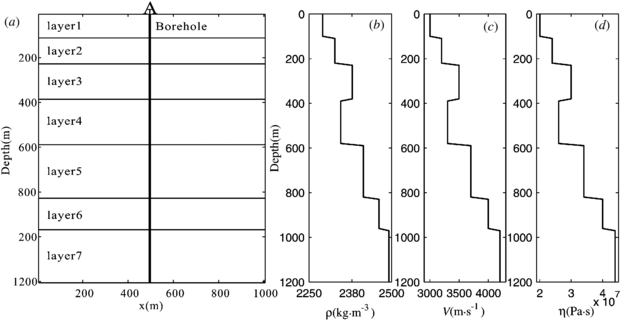
Figure 1. Model geometry (a) and true models for density (b), velocity (c), and viscosity coefficient (d).
Download figure:
Standard image High-resolution imageTable 1. True model values for the seven-layer model.
| Parameters/layer | 1 | 2 | 3 | 4 | 5 | 6 | 7 |
|---|---|---|---|---|---|---|---|
| h(m) | 100 | 120 | 160 | 200 | 240 | 140 | 240 |
| υ (m s–1) | 3000 | 3200 | 3500 | 3300 | 3700 | 4000 | 4200 |
| ρ (kg m–3) | 2291 | 2329 | 2381 | 2347 | 2415 | 2462 | 2492 |
| η (Pa s) | 2.0 × 10⁷ | 2.4 × 10⁷ | 3.0 × 10⁷ | 2.6 × 10⁷ | 3.4 × 10⁷ | 4.0 × 10⁷ | 4.4 × 10⁷ |
We test the variation in the misfit function on the seven-layer model by changing only the values of the sixth layer. Figure 2(a) is the misfit function curve of the relative variation to the true υ, and figure 2(b) is the misfit function curve of the relative variation to the true η. The relative variation is obtained by
where m is the changing model value and mtrue is the true model value.

Figure 2. (a) Misfit function of relative variation to the true velocity only and (b) misfit function of relative variation to true viscosity coefficient only.
Download figure:
Standard image High-resolution imageFigure 2(a) shows that the misfit function increases with increased difference between the true and changed velocities, which means that velocity has a high sensitivity in the data, as shown by the well-convex shape. For parameter η, the misfit function slowly varies when η is smaller than the true model, but significantly varies when η is higher than the true ones. For the same relative variation, the magnitude of the misfit function to υ is larger than that to η by a magnitude of 2–3, such as the relative variation 50% with a magnitude of 2. Thus, υ is much more sensitive than η to the misfit function.
3.2. Inversion strategies
In this section, we compare two inversion strategies, and the better one is used in subsequent numerical tests. As mentioned above, υ is more sensitive so we first try a one-by-one parameter inversion strategy. In the first step, we reconstruct only ρ and υ while fixing η as the initial model. In the second step, only η is rebuilt while ρ and υ are fixed as the reconstructed models in the first step. The seven-layer model shown in figures 1(b)–(d) is tested by using this inversion strategy. The initial models are homogeneous models with 2400 kg m−3, 3600 m s−1, and 3.4 × 10⁷ Pa s for density, velocity, and viscosity, respectively. Nine frequencies between 3.5 and 20 Hz are used, and the iteration number is 1000 for each frequency. Figure 3 shows the reconstructed results where ρ and υ well match the true models while η is a poor match. The reason is that the reconstructed ρ and υ do not well match the true models, and the errors caused by ρ and υ change into noise to η, which results in the poor convergence of η. The inverted models in figure 3 show that ρ and υ can be well reconstructed with η being the initial model, whereas η cannot be rebuilt with ρ and υ having some errors to the true models. The result reveals that η is more sensitive to noise than ρ and υ.
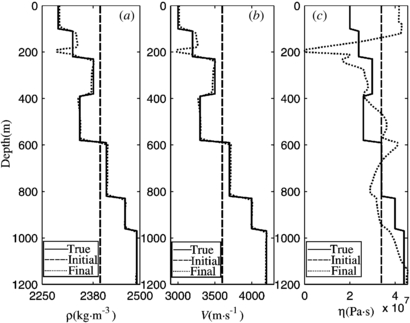
Figure 3. Reconstructed models for density (a), velocity (b), and viscosity coefficient (c) by using the one-by-one parameter inversion strategy. The true, initial and final models are plotted with solid (—), dash (—) and point (⋅⋅⋅) lines, respectively.
Download figure:
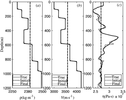
Standard image High-resolution imageThen, we try the second inversion strategy, namely, the joint inversion strategy. We reconstruct the three parameters jointly and obtain the step lengths by the parabolic fitting with (11)–(12). In the early inversion stage, υ is more sensitive than η, so ρ and υ are dominant and the step length is more suitable for them. As iteration is continued, ρ and υ become closer to the true models, and then η dominates and the step length becomes more appropriate forη. Consequently, ρ and υ can be well reconstructed in the early stage, whereas η can be well rebuilt in the later stage of inversion. We also test the joint inversion strategy on the seven-layer model in figures 1(b)–(d), and the parameters used in the inversion are the same as the ones in figure 3. Figure 4 shows that the reconstructed models are in agreement with the true models. In the following numerical tests, we adopt the joint inversion strategy.

Figure 4. Reconstructed models for density (a), velocity (b), and viscosity coefficient (c) by using the joint inversion strategy. The line depictions are the same as in figure 3.
Download figure:
Standard image High-resolution image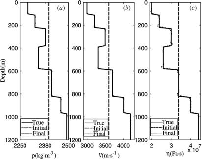
Figure 5. Reconstructed models for density (a), velocity (b), and viscosity coefficient (c) obtained by the Bunks frequency group strategy. The line depictions are the same as in figure 3.
Download figure:
Standard image High-resolution image4. Synthetic case studies
Based on the joint inversion strategy, we explore the ability and limitation of the current algorithm to recover the multi-parameter models. We compare three frequency-selection strategies and test the influences of initial models and the number of total iterations on the rebuilt models.
4.1. Comparisons between different frequency-selection strategies
To obtain global minimum solutions and improve the efficiency of waveform inversion, we compare three frequency-selection strategies. The first strategy, referred to as the single-frequency method (Brossier et al 2009, Kim et al 2011), is implemented one frequency by one frequency and from low to high frequency. The second strategy, referred to as the Bunks approach (Brossier et al 2009, Kim et al 2011), is an adaptation in the frequency domain of the time-domain approach of Bunks et al (1995). It consists of successive inversions of overlapping frequency groups. The third strategy, referred to as the group inversion approach (Brossier et al 2009), consists of successive inversions of slightly overlapping frequency groups.
In our study, we test and compare the three frequency selection strategies on the seven-layer model in figures 1(b)–(d). The initial models are homogeneous models with 2400 kg m−3, 3600 m s−1, and 3.4 × 10⁷ Pa s for density, velocity, and viscosity coefficient, respectively. The inverted frequencies for each frequency selection strategy are empirically selected as shown in table 2. The main frequency of the Ricker wavelet is 15 Hz, and the space interval is 10 m; 1 shot and 120 receivers are used for the zero-offset VSP test. The iteration number is 1000 for each frequency or frequency group. We compare the inversion times and accuracies of the final results of each strategy. The accuracy of the reconstructed model is assessed by the normalized model error (NME):
where M represents the parameters ρ, υ, and η; Mcal and Mtrue are the inverted and true models, respectively; and N is the total number of each parameter.
Table 2. Comparisons between the reconstructed models from three kinds of frequency-selection strategies.
| Frequency-selection strategies | Single | Bunks | Frequency groups |
|---|---|---|---|
| 1.57 | 1.57 | ||
| 3.53 | (1.57 3.53) | ||
| 5.49 | (1.57 3.53 5.49) | (1.57 3.53 5.49) | |
| Frequencies | 7.84 | (1.57 3.53 5.49 7.84) | (5.49 7.84 9.41) |
| 9.41 | (1.57 3.53⋅⋅⋅7.84 9.41) | (9.41 11.37 13.33) | |
| 11.37 | (1.57 3.53⋅⋅⋅9.41 11.37) | (13.33 15.29) | |
| 13.33 | (1.57 3.53⋅⋅⋅11.37 13.33) | ||
| 15.29 | (1.57 3.53⋅⋅⋅13.33 15.29) | ||
| Time (minutes) | 46.07 | 197.50 | 67.73 |
| NME of ρ | 9.88 × 10⁻⁴ | 8.82 × 10⁻⁴ | 0.0014 |
| NME of υ | 0.004 | 0.0035 | 0.0056 |
| NME of η | 0.0208 | 0.0187 | 0.0289 |
Figures 4–6 show the reconstructed models for the single-frequency approach, Bunks approach, and group inversion approach, respectively. Table 2 shows the accuracies of the final models and calculation time for three frequency-selection strategies. Given the sufficiently large iterations, the reconstructed models of ρ, υ, and η well match the true models. Table 2 shows that the highest accuracies of the final results are 8.82 × 10⁻⁴, 0.0035, and 0.0187 for ρ, υ, and η by using the Bunks approach. However, this approach is the most time consuming one at 197.5 minutes, which is about four times the inversion time for the single-frequency method (46.07 minutes) and about three times the calculation time for the frequency group approach (67.73 minutes). The accuracies of the final models by the single-frequency method (i.e. 9.88 × 10⁻⁴, 0.004, and 0.0208 for ρ, υ, and η, respectively) are close to the accuracies by the Bunks approach but less time consuming. The accuracies (0.0014, 0.0056, and 0.0289 for ρ, υ, and η, respectively) and inversion time of the group inversion approach lies between the Bunks approach and the single-frequency approach. Considering the accuracies and calculation time without parallel implementation, we believe the single-frequency approach is preferred.

Figure 6. Reconstructed models for density (a), velocity (b), and viscosity coefficient (c) obtained by the frequency group strategy. The line depictions are the same as in figure 3.
Download figure:
Standard image High-resolution imageTo demonstrate further that the inverted models match the true models, we present the responses to the true, initial, and final models in figure 3. The time forward modelling is computed by finite difference in time domain, where the discrete pattern and PML boundary are the same as frequency domain modelling. The seismographs are recorded in 0.7 s, as shown in figure 7. Figure 7(a) is the response to the true models without considering the attenuation, whereas figure 7(b) is for the true model with attenuation. Clearly, the wave energy with attenuation is weaker than that without attenuation. Figures 7(b), (d) and (f) show that the seismograph for the final models is close to the one for the true models, which means that the reconstructed models are reliable and the inversion strategy used is feasible.
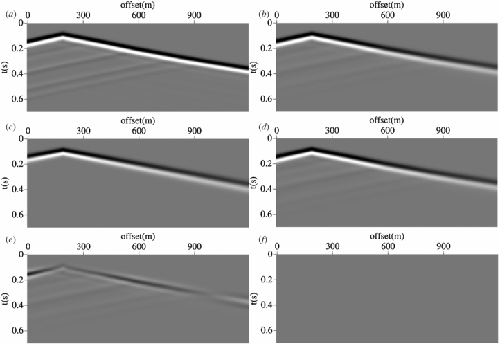
Figure 7. The responses to the true models with the viscosity efficient equal to zero (a), true models (b), initial models (c), and final models (d) as well as their corresponding residuals, where (e) is for the residuals between the response to the true models and to the initial models and (f) is for the residuals between the response to the true models and to the final models. The true, initial, and final models are plotted in figure 3. All the responses are plotted in the same scale.
Download figure:
Standard image High-resolution image4.2. Influences of the initial models on the final models
To assess the influence of the initial models on the final models, we compare two initial models. One is the 70-point smoothing of the true models in figures 1(b)–(d) and the other is the homogeneous models with 2600 kg m−3, 5000 m s−1, and 5.0 × 10⁷ Pa s for density, velocity, and viscosity coefficient, respectively. The single-frequency approach is used, and the inverted frequencies are the same as the ones in table 2 for this approach. The iteration number is 500 for each frequency. The true model is shown in figures 1(b)–(d). Figures 8 and 9 are the final models for the 70-point smoothing initial models and the homogeneous initial ones. The accuracies of ρ, υ, and η are 0.0014, 0.0055, and 0.0236 for the 70-point smoothing initial models. For the homogeneous initial models, the accuracies are 0.0014, 0.0055, and 0.0226, respectively. We can observe that the differences between the final models for the 70-point smoothing initial models and homogeneous initial ones are so small that they can be ignored. We can conclude that the influences of the initial models on the final results are small.
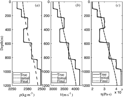
Figure 8. Reconstructed models for density (a), velocity (b), and viscosity coefficient (c) with the initial models obtained by smoothing the true models with 70 points. The line depictions are the same as in figure 3.
Download figure:
Standard image High-resolution image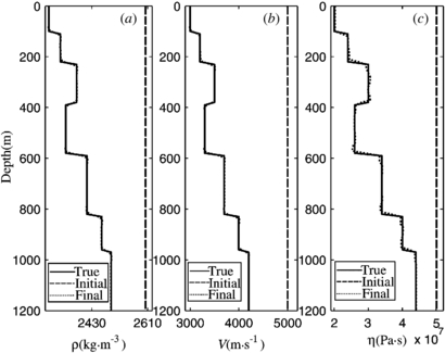
Figure 9. Reconstructed models for density (a), velocity (b), and viscosity coefficient (c) with homogeneous initial models. The line depictions are the same as in figure 3.
Download figure:
Standard image High-resolution image4.3. Influences of inverted frequencies and iterations on the final models
To determine the influences of inverted frequencies and the total number of iterations on the final results, we compare the final results with different frequencies and iterations. In this comparison, the true models of ρ and υ are the same as the ones in figures 1(b) and (c). However, the true model of η differs from the one in figure 1(d), which is modified from the VSP example of SEISCOPE (Operto et al 2007). The initial models are homogeneous models with 2400 kg m−3, 3600 m s−1, and 2.7 × 10⁷ Pa s for ρ, υ, and η, respectively.
We first compare the results of 500 iterations (figure 10) with 1000 iterations (figure 11), where four inverted frequencies (1.57, 3.53, 5.49, and 7.84 Hz) are used. The accuracies of ρ, υ, and η with 500 iterations are 0.0015, 0.0061, and 0.0204, respectively, whereas the accuracies with 1000 iterations are 0.0046, 0.0012, and 0.0153, respectively. The differences in the inverted ρ and υ between the two iterations are small, whereas the difference in η is large, especially in the position of layer stripping. We can observe that larger iterations result in better reconstruction of η, which means that η is more dependent on the iterations.
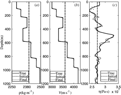
Figure 10. Reconstructed models for density (a), velocity (b), and viscosity coefficient (c) with 4 frequencies and 500 iterations for each frequency. The line depictions are the same as in figure 3.
Download figure:
Standard image High-resolution image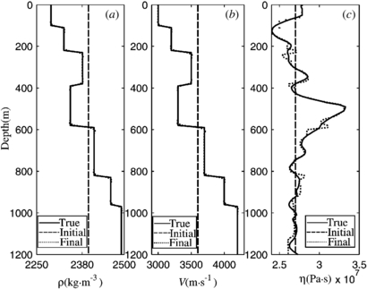
Figure 11. Reconstructed models for density (a), velocity (b), and viscosity coefficient (c) with 4 frequencies and 1000 iterations for each frequency. The line depictions are the same as in figure 3.
Download figure:
Standard image High-resolution imageWe then compare the final models from four inverted frequencies (figure 10) with the ones obtained by eight inverted frequencies (figure 12), which are the same as the ones in table 2 for the single-frequency strategy. In both cases, the iteration number is 500. The accuracies of ρ, υ, and η with eight frequencies are 0.0013, 0.0051, and 0.0174, respectively. Table 3 compares the accuracies of the two kinds of frequencies, and the results with eight frequencies and 500 iterations are much better. We then compare the final models by 1000 iterations and four inverted frequencies with the ones by 500 iterations and eight inverted frequencies, and results show that they have close inversion accuracies.
Figure 12. Reconstructed models for density (a), velocity (b), and viscosity coefficient (c) with 8 frequencies and 500 iterations for each frequency. The line depictions are the same as in figure 3.
Download figure:
Standard image High-resolution image
Table 3. Final models of different numbers of frequencies and iterations.
| Number of frequencies | Number of iteration | NME of ρ | NME of υ | NME of η |
|---|---|---|---|---|
| 4 | 500 | 0.0015 | 0.0061 | 0.0204 |
| 4 | 1000 | 0.0012 | 0.0046 | 0.0153 |
| 8 | 500 | 0.0013 | 0.0051 | 0.0174 |
From table 3 and figures 10–12, we can conclude that the total number of iterations, i.e. the number of inverted frequencies multiplied by the number of iterations, plays an important role in obtaining high-accuracy final models. When fewer inverted frequencies exist, we can improve the final models by increasing the number of iterations, and for more frequencies the final models can be well rebuilt with less iteration.
5. Conclusions
We have presented a joint inversion method to reconstruct density, velocity, and viscosity coefficient jointly from zero-offset VSP data by frequency-domain FWI. Among the three parameters, density and velocity are more sensitive to the misfit function than the viscosity coefficient. Moreover, density and velocity can be stably reconstructed even when the viscosity coefficient remains as the initial values.
Our inversion strategy mainly focuses on the updates of velocity and density in the early stage, whereas the viscosity coefficient is mainly rebuilt in the later stage. The inverted results of the early stage can supply better initial models for later density, velocity, and viscosity coefficient inversion, especially for viscosity coefficient inversion. Viscosity coefficient depends on iterations; thus, more iterations are preferred for obtaining inverted results that well match true models.
Through comparison with three frequency-selection strategies, we believe that the single-frequency approach outperforms the Bunks approach and group inversion approach without considering parallel computation. The influences of different initial models on the final models are tested, and the comparison shows that the algorithm is stable and not highly dependent on the initial models when the iteration is sufficiently large. Within some frequency range, a larger total number of iterations results in better final inverted results.
Acknowledgments
This study was supported by the National Natural Science Foundation of China (grant no 40974054), the National Basic Research Program of China (grant no 2009CB219301), the National Public Benefit Scientific Research Foundation of China (grant no 201011078), the National Innovation Research Project for Exploration and Construction of Oil Shale (grants no OSP-02 and OSR-02), and Project 20121065 supported by the Graduate Innovation Fund of Jilin University. We also thank the two anonymous referees for their valuable suggestions for improving this paper.