
Abstract
Recently, several studies have started to explore covert visuospatial attention as a control signal for brain–computer interfaces (BCIs). Covert visuospatial attention represents the ability to change the focus of attention from one point in the space without overt eye movements. Nevertheless, the full potential and possible applications of this paradigm remain relatively unexplored. Voluntary covert visuospatial attention might allow a more natural and intuitive interaction with real environments as neither stimulation nor gazing is required. In order to identify brain correlates of covert visuospatial attention, classical approaches usually rely on the whole α-band over long time intervals. In this work, we propose a more detailed analysis in the frequency and time domains to enhance classification performance. In particular, we investigate the contribution of α sub-bands and the role of time intervals in carrying information about visual attention. Previous neurophysiological studies have already highlighted the role of temporal dynamics in attention mechanisms. However, these important aspects are not yet exploited in BCI. In this work, we studied different methods that explicitly cope with the natural brain dynamics during visuospatial attention tasks in order to enhance BCI robustness and classification performances. Results with ten healthy subjects demonstrate that our approach identifies spectro-temporal patterns that outperform the state-of-the-art classification method. On average, our time-dependent classification reaches 0.74 ± 0.03 of the area under the ROC (receiver operating characteristic) curve (AUC) value with an increase of 12.3% with respect to standard methods (0.65 ± 0.4). In addition, the proposed approach allows faster classification (<1 instead of 3 s), without compromising performances. Finally, our analysis highlights the fact that discriminant patterns are not stable for the whole trial period but are changing over short time intervals. These results support the hypothesis that visual attention information is actually indexed by subject-specific α sub-bands and is time dependent.
Export citation and abstract BibTeX RIS
1. Introduction
Covert visuospatial attention represents the ability to focus attention at one point in space without overt eye movements [1]. Recent studies have started to exploit covert visuospatial attention as a control signal for brain–computer interface (BCI). These studies demonstrated that subjects can modulate both the visual responses elicited by external stimuli and the excitability of their visual cortex in a fully endogenous way. The former modality is mainly based on steady-state visual evoked potential paradigms, where subjects are instructed to focus their attention on lights flickering at predefined frequencies. Although BCIs relying on external stimulation may reach good classification accuracy [2, 3], these paradigms might be tiring and irritating, especially over long periods of time.
A much more flexible and spontaneous approach is to exploit voluntary covert visual attention whereby neither stimulation nor gazing is required. This approach fits especially well in a navigation task when BCI is used to control devices (i.e. a telepresence robot or a wheelchair) in a natural environment. In this framework, the BCI user could command the device to turn by spontaneously orienting his/her attention to a particular location in space.
Different neurophysiological studies have demonstrated the involvement of α-band in voluntary visual attention tasks [4–8]. Usually, subjects are instructed to focus attention at one specific location in space indicated by a cue. The related synchronization of the α-band in the parieto-occipital regions seems to reflect an inhibition mechanism in the retinotopical spatial organization of the visual cortex. In particular, Rihs et al [6] demonstrated that this behavior is highly selective and topographically specific with respect to the attended locations (e.g., in the case of two lateralized locations, an ipsilateral α synchronization occurs in order to suppress irrelevant stimuli in the unattended side of the visual field). BCIs based on covert visuospatial attention exploit these changes in α-power in order to discriminate over two or more attended locations [9–11].
Nevertheless, the full potential of this BCI paradigm remains relatively unexplored. In fact, standard methods do not take into consideration the possible modulations of α sub-bands, nor the time evolution of the signals after the instructional cue.
The aim of this study is to compare different analysis methods to exploit covert visual attention in BCI. Therefore, we propose four different analysis approaches. Starting from the standard method, firstly we increase the frequency resolution within the α-band. The intuition is that only sub-bands are carrying discriminative information as is the case of sensory-semantic and memory processes [12] and the modulation of μ-rhythms during motor imagination tasks [13]. To our knowledge, this is the first time a voluntary modulation of α sub-bands has been taken into account for covert visuospatial attention. Secondly, we hypothesize that attention-related patterns are evolving over time and consequently a time-dependent approach would enhance BCI performances. Previous neurophysiological studies have already highlighted the role of temporal dynamics in attention mechanisms [7, 14–19]. However, these important aspects are not yet exploited in the current BCI systems. In this work, we studied different methods that explicitly cope with the natural brain dynamics during visuospatial attention tasks in order to enhance BCI robustness and classification performances.
2. Data collection
2.1. Participants
Ten healthy volunteers (age 27.6 ± 1.7; three female; eight right handed) participated in this study. All participants had normal or corrected-to-normal vision. No attention problems have been reported. Subjects did not have any previous experience with covert visuospatial attention paradigms. The study was approved by the local ethics committee and carried out in accordance with the principle of the Declaration of Helsinki.
2.2. Visual paradigm and task
In this study, we exploited a visual attention paradigm based on two target locations (left and right). A white fixation cross in the middle of the screen (size 3.12°) and two circles (to-be-attended locations) at the bottom-left and bottom-right positions (distance 12°, size 3.12°) were displayed continuously. At the beginning of each trial, participants were instructed to gaze at the fixation cross. After 2000 ms (fixation period), a green symbolic cue (size 3.12°) appeared at the middle of the screen for 100 ms (cue period). The participants had to focus their attention on the to-be-attended location indicated by the cue, without moving the eyes (covert attention period). After a random time between 3000–5000 ms, a red target (size 3.12°) appeared always at the correct target location for 1000 ms (target period) to inform participants of the trial end. No additional discrimination task was required on the red target. Participants were instructed to blink (if necessary) only after the target appeared. Note that in this work we restricted the analysis period until 3000 ms after the cue in order to avoid any visual evoked stimulation. Figure 1 shows the schematic representation of the protocol with the time intervals adopted.

Figure 1. Schematic trial representation. The fixation period starts 2000 ms before the cue. The cue (100 ms duration) indicated the side where to focus attention. After 3000–5000 ms, the circle corresponding to the correct target location becomes red (for 1000 ms). The analysis period lasted for 3000 ms. In the figure, the cue and the red circle are larger than in reality for visualization purposes.
Download figure:
Standard imageThe visual layout was based on previous works both in neurophysiological [6, 7, 20] and in BCI studies [9–11]. Specifically, the choice of the target positions (angle and distance) was made to exploit the retinotopical organization of the visual cortex to obtain robust scalp signals [21].
Each participant performed a total of 200 trials in five different runs on the same day (session). The mean duration of each run was 6.06 ± 0.14 min. After each run, participants had a break of 5 min. Equal numbers of stimuli for both classes (left and right) were randomly presented.
2.3. Electrooculogram artifact removal
The electrooculogram (EOG) was recorded by means of three electrodes: two placed either side of the eyes and one at the glabella. Vertical and horizontal EOG components were computed with a bipolar derivation in the frequency range of 1–7 Hz (Butterworth filter, order 3). We manually discarded trials where any of the two EOG components had an amplitude higher than 50 μV. The average number of discarded trials across subjects was 15.6% ± 7.8% (equally distributed over the two classes and runs).
2.4. EEG data acquisition and processing
Signals were acquired with an active 64-channel EEG system (Biosemi, Amsterdam, Netherlands) at 2048 Hz. The 64 electrodes were placed according to the standard international 10–20 system. Data were downsampled at 512 Hz and the dc component was removed. A Laplacian spatial filter was applied to the data in order to highlight the activity of the local sources. We used a configuration based on eight neighbors weighting the contribution of each neighbor according to the distance from the target electrode. The aforementioned montage represents an extension of the standard Laplacian configuration reported in the literature [22]. Afterward, in each trial we selected the analysis period (up to 3000 ms after the cue, see figure 1). No baseline correction was computed on the signals.
In order to analyze the α-band in more detail (compared to the literature), we applied seven narrow band-pass filters (Butterworth filter, order 4, 3 Hz band window) centered at the frequencies at integer values between 8 and 14 Hz. Based on the literature [5–7, 20], we preselected channels in the parieto-occipital regions of the brain (electrodes P7–8, PO7–8, O1–2). For each frequency-channel pair (defined as a feature), we computed the envelope of the signal by using the absolute value of the Hilbert transform.
3. Methods
The role of the α-power in covert visual attention tasks has already been reported in many works [5, 6, 10, 23]. Previous analyses only considered the whole α-band and whole attention period (time independent) in order to classify visual attention tasks. The main aim of this work is to understand how features evolve over time and to explore different approaches to increase classification accuracy of this specific mental task. In this section, we first present the analysis and the statistical validation of the temporal evolution of the features. Secondly, we describe the peculiarities of the four different proposed approaches. Finally, we report the feature selection and classification methods applied for each of them.
3.1. Feature evolution over time
Despite grand average studies that show a constant ipsilateral activation over the whole trial period, this might not be the case for single trial analysis. A key aspect is to understand how the most discriminant features evolve over time and if it is possible to identify intervals sharing common patterns. First of all, for each frequency-channel pair, we used the Fisher score value in order to identify the most discriminant features over the two classes (left and right visual attention) sample by sample and, for each sample, we selected those features that contributed at least 15% to the overall sum. This procedure allowed us to identify the sets of most discriminant features over the whole trial period. Then, in order to study the stability of a given set, we defined a consistency index that compares the set of features selected at time t, Ωt, with those selected in the rest of the trial Ωj (with j ≠ t). Given a set Ωt, the consistency index ρt is computed for each time point, or sample, based on the formula

The index ρt shows the proportion of features selected at time t that recurs in the rest of the trial. More generally, it describes temporal clusters that share a common set of discriminant features.
We validated the most prominent clusters (time intervals sharing at least half of the discriminant features) with a non-parametric statistical test [24]. Random data were generated from multivariate uniform distributions for the two task conditions (attending left and right) for all channels and frequency bands. The same procedure applied for real EEG data was used to select the most discriminant features at each time point on this random dataset. Clusters were selected based on adjacent pixels with a ρ value greater than 0.5 (sets sharing half of discriminant features). For each cluster, we sum its weight. We performed 500 repetitions of this procedure. The largest cluster sum was taken for each repetition to obtain an empirical random distribution of the cluster weights. Finally, only those clusters from the EEG data whose weights were above 99% of the random distribution were considered statistically relevant (p < 0.01).
3.2. The four different approaches
Firstly, we studied the contribution of α sub-bands in carrying visual attention information, by increasing the resolution in the given frequency range. Secondly, we focused on the evolution of the features over time. Splitting the attention period into consecutive, non-overlapping, windows (of 150 ms [14]) allowed us to perform a time-dependent feature selection and classification. In particular, the selected window length ensured at least one complete oscillation of each analyzed frequency, i.e. 1.2 and 2.1 oscillation cycles at the lowest (8 Hz) and highest (14 Hz) frequency bands. By comparing the different approaches, we expect to have a better understanding of the best method to classify covert visuospatial attention.
Table 1 summarizes the four different approaches explored in this study. In the case of A0, we replicated the standard method generally used in the literature, where we computed one single feature per channel representing the whole α-band power over the whole attention period [9, 10]. In this approach, any time information was discarded. In A1, we performed a more detailed frequency analysis (seven α sub-bands) while keeping the same time window for comparison purposes. In A2, we still used the whole attention period for selecting features and training the classifier as in A1. However, we investigated the performances of this classifier if tested on different time windows. Finally, in A3 we used a fully time-dependent approach by selecting features and training the classifier for each time window.
Table 1. The four different approaches studied in this work. Whole period refers to analysis computed for the entire attention period (0–3000 ms). Time windows correspond to analysis computed separately for each interval. In the case of A0, an additional frequency average was performed.
| Frequency resolution | Feature selection | Classification training | Classification testing | |
|---|---|---|---|---|
| A0 | α-band | Whole period | Whole period | Whole period |
| A1 | α sub-bands | Whole period | Whole period | Whole period |
| A2 | α sub-bands | Whole period | Whole period | Time windows |
| A3 | α sub-bands | Time windows | Time windows | Time windows |
To test the different approaches we did a five-fold cross validation where the dataset was split five times into 80% for feature selection and training and 20% for testing. The independence between training and testing sets ensured avoiding the circularity problem [25]. Figure 2 illustrates schematically the analysis method. The following sections provide more details about each step.
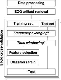
Figure 2. Data were processed in order to extract the envelope of the signal in seven α sub-bands. Trials with EOG activity were discarded. The dataset was split in training and test set with a five-fold cross validation. According to the approach (A0–A3) frequency and time averaging (*) was performed independently on the training and test set. The training set was used to select the most discriminant features and to train the classifiers. Finally, the test set was used for performance evaluation.
Download figure:
Standard image3.3. Feature selection and classification
First of all, we computed the Fisher score value of each feature in the whole attention period (approaches A0, A1 and A2) or in different time intervals (approach A3). The features that contribute more than 15% to the overall sum (of the whole attention period or of each time interval) were selected as input for classification. Note that for A0, A1 and A2, the selection was totally time-independent since data were averaged over the whole trial period (0–3000 ms). Conversely, in the case of A3, we performed a separate time-dependent selection in each time window (150 ms).
The features selected in the previous step were used as an input to a quadratic discriminant analysis (QDA) with a diagonal covariance matrix estimation. For the time-independent approaches (A0, A1 and A2), one single classifier was trained with data of the whole attention period and tested globally (A0, A1) or locally (A2) in each time window. In the case of the fully time-dependent approach (A3), we trained a separate classifier for each time window. Then each classifier was tested separately in its own interval. The dimensionality of the classifiers was equal to the number of features selected (see table 3) and varies across subjects, approaches and time windows (in the case of approach A3).
In order to evaluate classification performances under the different conditions, we used the area under the ROC (receiver operating characteristic) curve (AUC) value and its standard error computed according to [26]. In the case of A2 and A3, we computed the AUC per window in order to evaluate the classifier(s) response in each time interval.
4. Results
In this section, we first present the time evolution of signals during the visual attention period averaged across subjects. Secondly, we report the evolution and consistency over time of the discriminant features. Finally, we compare the number of features selected and the classification results for the four aforementioned methods (A0, A1, A2, A3).
4.1. Grand average behavior
Topographic maps in figure 3 show the evolution of the envelope of the signal (grand average over all subjects) in the α-band for different time windows. The maps represent the difference between the two conditions (focusing attention on the right versus left targets). An ipsilateral synchronization with respect to the mental task is evident in the parieto-occipital regions. The synchronization appears from 600 ms after cue and holds until the end of the attention period (3000 ms). The activity appears to be strongly lateralized. Table 2 depicts the p-values computed using a paired-sample t-test under the two conditions (left and right attention) for each time interval and channel. Statistically significant differences for most of the channels occur from 600 ms after the cue. These results are in line with previous studies [6, 7, 10, 23].

Figure 3. The evolution of the envelope of the signals in the α-band (8–14 Hz). The topographic maps represent the difference between two attention conditions (attending to the right or to the left) in six different time windows. The signals were averaged across subjects.
Download figure:
Standard imageTable 2. The evolution of the p-values computed using a paired-sample t-test under the two conditions over the trial period and for a subset of parieto-occipital channels. Statistically significant results are reported in bold.
| Time intervals (s) | ||||||
|---|---|---|---|---|---|---|
| Channels | −0.3 to −0.15 | 0.0–0.15 | 0.6–0.75 | 0.9–1.05 | 1.8–1.95 | 2.7–2.85 |
| PO7 | 0.24 | 0.41 | <0.05 | <0.05 | <0.05 | <0.05 |
| PO3 | 0.73 | 0.12 | <0.05 | <0.05 | <0.05 | <0.05 |
| O1 | 0.64 | 0.06 | <0.05 | 0.07 | 0.39 | 0.09 |
| POz | 0.37 | 0.22 | <0.05 | <0.05 | <0.05 | <0.05 |
| Oz | 0.58 | 0.42 | 0.55 | 0.08 | 0.12 | <0.05 |
| O2 | 0.34 | 0.64 | <0.05 | <0.05 | 0.42 | <0.05 |
| PO4 | 0.51 | 0.11 | 0.21 | <0.05 | <0.05 | <0.05 |
| PO8 | 0.14 | <0.05 | <0.05 | <0.05 | <0.05 | <0.05 |
4.2. Feature evolution over time
Figure 4 depicts the consistency index for each subject, which reflects the proportion of features in a given set (vertical axis) that are also present in other time points. Values are normalized between 0 (blue) and 1 (red). As shown in figure 4, sets of features are clustered in time intervals. Statistically significant clusters (p < 0.01) are highlighted with a black border. The non-parametric statistical test has been performed with respect to set of features selected from random data.

Figure 4. The consistency over time of the sets of selected features. The color code reflects the degree to which two samples share common features. Blue means that no features are in common; red means that the two samples are sharing the same features. The value is normalized between 0 and 1.
Download figure:
Standard imageThe first and most important outcome is that none of the subjects showed a stable set of discriminant features over the whole trial period. In fact, for all subjects only short time intervals where features are consistent can be identified. Interestingly, these intervals seem to have different lengths and occur at different times across subjects. Furthermore, features selected later (after ∼1500 ms) are generally stable until the end of the trial (i.e. subjects s1, s4 and s6). For instance, for subject s1 the set of features selected at t = 1000 ms (vertical axis) are highly discriminant only for a short interval centered at this time point. In addition, features selected at t > 2000 ms are consistent until the end of the trial (along the horizontal axis). Conversely, for subject s10 the feature discriminability presents a different temporal dynamic. In fact, for this subject only short time windows sharing the same features can be identified in the whole trial period (0–3000 ms). This behavior is in line with previous studies [6, 9, 10].
These findings support our hypothesis of an evolving pattern during a visual attention task, which represents the main motivation for a time-dependent approach.
4.3. Number of features selected
The number of selected features varies across subjects and approaches. Table 3 illustrates the minimum, maximum and average number of features selected in each approach. In particular, for A3 each time window is considered. Note that in the case of A0, the original number of features was 17 (number of channels) while for the other approaches was 119 (channels × frequency bands). Since the number of features determines the dimensionality of the classifier, it is worth noting that the number of features after selection is similar for approaches A1, A2 and A3.
Table 3. Minimum, maximum and averaged number of features selected across subjects and approaches. In the case of A3 each window within the trial period was considered. The total number of possible features before selection was 17 (number of channels) for A0 and 119 (channels × frequency bands) for the other approaches.
| No. of selected features | |||
|---|---|---|---|
| Minimum | Maximum | Average | |
| A0 | 1 | 3 | 1.9 |
| A1 | 7 | 13 | 9.7 |
| A2 | 7 | 13 | 9.7 |
| A3 | 7 | 8 | 7.9 |
4.4. Comparison of classification performances
In figure 5, we report the comparison for the four aforementioned methods. In the case of A2 and A3, where we tested the classifiers over time windows, the maximum AUC is reported. The first outcome is that just by increasing the frequency resolution (from A0 to A1) AUC reaches on average 0.70 ± 0.04, corresponding to an increase of 6.5% ± 2.7%. Individually, the increment can be more dramatic as in the case of s3, s4, s7 and s10 where we report a gain of 11.9%, 16.6%, 12.5% and 22.0%, respectively.
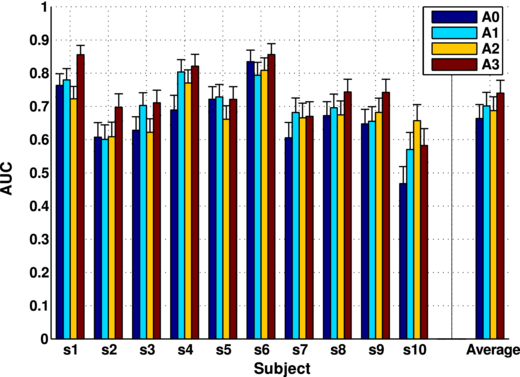
Figure 5. AUC comparison between the four different approaches (A0–A3) for each subject with the standard error. Maximum AUC over time is reported for A2 and A3 approaches.
Download figure:
Standard imageFurthermore, our results demonstrate that a fully time-dependent approach (A3) achieves the highest performances. The best AUC is observed for subject s6 (0.86±0.03) and the worst for s10 (0.59±0.05). As depicted in figure 5, approach A3 improved the performance of every subject compared to the current state-of-the-art approach A0. On average, the AUC value reaches 0.74±0.03 with an increase of 12.3% ± 2.3%. Table 4 reports the averaged gain of each method with respect to the other approaches in more detail.
Table 4. Comparison of averaged performances, with standard error, for each approach with respect to the others. Columns represent the reference approach, rows the compared one. Positive values correspond to an increment in classification performances measured by AUC. Increments indicated in bold are statistically significant (p < 0.05).
| A0 | A1 | A2 | |
|---|---|---|---|
| A1 | 6.5% ± 2.7% | ||
| A2 | 5.0% ± 4.4% | −1.5% ± 2.4% | |
| A3 | 12.3% ± 2.3% | 5.6% ± 1.9% | 7.7% ± 2.6% |
It is worth noting that the performance of A3 is statistically superior to all other methods. Likewise, the difference in the performance of A1 with respect to A0 is statistically significant. The comparison has been validated with a paired, two-side Wilcoxon statistical test (p < 0.05).
In figure 6(a) we present the time evolution of the AUC in the two time-dependent approaches A2 and A3 averaged across subjects. Both curves quickly increase in the first second and stabilize for the rest of the attention period. With approach A3 the AUC reaches a higher value (as already expected from figure 5) but in less time. The performance increment of approach A3 is statistically significant.

Figure 6. (a) Time evolution of the AUC for A2 and A3 approaches. The AUC is averaged across all subjects and standard error is reported (shadowed area). (b) Time needed for approaches A2, A3 to reach the same AUC level as approach A0. When that level is not reached, time to reach the maximum is reported (* in the plot).
Download figure:
Standard imageIn figure 6(b) we show the time needed for approaches A2 and A3 to reach the same AUC level as approach A0. Also in this case, the fully time-dependent approach is more than 2 s faster (on average) with respect to the whole classification period (approach A0). In other words, we can reach the same level of performance as in the literature, within only 1 s instead of 3 s. This provides further evidence that time-dependent classifiers can capture better and faster the evolution of the signals in a visual attention task.
5. Discussion
In order to determine the best method for single trial classification of covert visuospatial attention we have compared four different approaches. Starting from a classical approach where data have been studied in the α-band (8–14 Hz) and in a broad time period, as in the literature [4–6, 8–10, 20], we performed a more detailed analysis in both time and frequency domains in order to better investigate the evolution of the patterns involved in visual attention tasks.
Analysis on the grand average (figure 3) shows an ipsilateral increment of the α-power in the parieto-occipital regions, which is coherent with the literature [5, 6, 10]. However, the comparison between A0 and A1 suggests that only selective sub-bands of the whole α-band are discriminative and informative for classification. Based on these findings, we hypothesize that the well-known contribution of α-power during attention represents, in fact, a voluntary modulation of particular α sub-bands. Although many works studied covert visual attention mechanism in the broadband frequency range (from δ- to γ-bands) [27–31], to our knowledge this is the first time sub-bands of α are examined separately. Moreover, these results are in line with previous neurophysiological studies on the role of individual α frequencies in sensory-semantic and memory processes [12].
Increasing frequency resolution is not the only way to reach better classification performances, as demonstrated by approaches A2 and A3. Time evolution of the signals seems to play a significant role in visual attention tasks. Evidence from different studies [7, 14–19] seems to identify temporal aspects in visual attention mechanisms. In particular, two temporal phases are generally highlighted in these works: shift and sustained attention phases. Analysis on the feature distribution over time (figure 4) supports this conclusion. First of all, none of the subjects exhibited any set of features that were stable for the whole trial period. Second, for most of the subjects (i.e. s1, s2, s4, s5, s6, s7) late periods in the trial are characterized by more consistent discriminant features, which may correspond to the sustained phase of attention. Nevertheless, in figure 4 we show the possibility of identifying even earlier time intervals with stable patterns in most cases (e.g., for subjects s1–8), probably related to the shift of attention. Furthermore, our temporal analysis gives us the possibility of tracking the patterns evolution also within these rather stable phases (as in the case of subjects s1, s4 and s6). We can hypothesize that these intervals of stability reflect the natural time-course of a top–down visual attention task [7, 16, 32]. Future work will be devoted to the study of the nature of these stable features in order to verify the temporal involvement of specific α sub-bands and brain regions.
The possibility of identifying different phases during covert visuospatial attention tasks supports our intuition of a time-dependent approach for feature selection and classification. In fact, our classification results suggest that A3 can track data evolution over time better than other approaches, yielding a higher classification performance in less time. Moreover, the selection of optimal time windows (subject by subject) might further enhance performance. In fact, as shown in figure 4, time intervals with stable features can have different length and occur at different times. Similarly, the best classification intervals are specific for each subject. We hypothesize two reasons for this: on one hand it might depend on different visuospatial paths followed by subjects to reach the final locus of attention (target location). This hypothesis is supported by the well-known retinotopical spatial organization of the visual cortex [6, 9, 11]. On the other hand, it may be due to the individual's ability to maintain attention over long periods of time. As a matter of fact, figure 4 shows that only four subjects out of ten are able to generate discriminable and consistent features at the end of the trial (s1, s4, s6 and s7). Nevertheless, the classification accuracy reported in figure 5 shows that our time-dependent approach A3 can deal with possible fluctuations of attention better than standard approach A0.
In addition, both temporal analysis and classification performances show that our approach is not biased by the cue stimulus. In fact, in figure 4 none of the subjects presents early intervals (before ∼500 ms) with significant stable features. Moreover, the best classification intervals occur only after ∼500 ms of the beginning of the trial (figure 6). These results support the robustness of our method with respect to evoked potentials driven by the cue stimulus.
Generally, the average increase in performance of our time-dependent approach A3 (12.3 ± 2.3% with respect to A0) is a fundamental improvement, which could allow covert visual attention to be used as a viable control signal for BCI. In addition, the described method is fully compliant with the requirements for an online implementation. Moreover, the short time (30 min on average) needed to train a subject is in line with other classical BCI paradigms using voluntary modulation of brain activity (i.e. μ-rhythm modulation for motor imagery-based BCI [33, 34]). The next challenge is to demonstrate that subjects can learn how to better modulate their α activity over sessions. This learning effect was demonstrated in classical motor imagery BCIs [35–37], but there is currently no evidence in the literature for covert visual attention.
A fully time-dependent approach such as A3 seems to be the best method for covert visuospatial attention classification. However, the main drawback of this approach is that it is designed to fit synchronous protocols, since the time localization plays an important role for classification. This might be a limitation in some BCI applications where a continuous and asynchronous control is required (i.e. brain-controlled robots and neuroprostheses [33, 34, 38, 39]). Nevertheless, our fully time-dependent approach (A3) can still be applied in asynchronous paradigm where subject's attention is cyclically forced back to the center of the screen after delivering each mental command. This solution allows us to cope with the natural brain dynamics in visuospatial attention task ensuring high classification performances and without compromising the continuous control required by the application.
6. Conclusion
This study suggests that single trial classification of covert visuospatial attention may be enhanced by a more detailed analysis both in the frequency and time domains. We propose a new method that relies on α sub-bands and time-dependent classification. For the first time, we have demonstrated that modulations of α sub-bands during covert visuospatial attention can be successfully exploited to increase BCI classification accuracy. Moreover, our time-dependent approach can capture the temporal dynamics of visual attention already reported in the literature. In this respect, this method allows the decoding of visual attention despite the fact that the subject cannot sustain stable patterns of brain activity over the whole attention period. Finally, this approach assures good classification performances for all subjects and—more importantly—leads to an increase of 12.3% (on average) with respect to classical methods reported in the literature.
Acknowledgments
This work is supported by the European ICT Programme Project TOBI (FP7-224631). This paper only reflects the authors' views and funding agencies are not liable for any use that may be made of the information contained herein.