


ABSTRACT
Stellar binary systems, specifically those that present the most accurate available orbital elements, are a reliable tool to test the accuracy of astrometric observations. We selected all 35 binaries with these characteristics. Our objective is to provide standard uncertainties for the positions and parallaxes measured by Hipparcos relative to this trustworthy set, as well as to check supposed correlations between several parameters (measurement residuals, positions, magnitudes, and parallaxes). In addition, using the high-confidence subset of visual–spectroscopic binaries, we implemented a validation test of the Hipparcos trigonometric parallaxes of binary systems that allowed the evaluation of their reliability. Standard and non-standard statistical analysis techniques were applied in order to achieve well-founded conclusions. In particular, errors-in-variables models such as the total least-squares method were used to validate Hipparcos parallaxes by comparison with those obtained directly from the orbital elements. Previously, we executed Thompsonʼs τ technique in order to detect suspected outliers in the data. Furthermore, several statistical hypothesis tests were carried out to verify if our results were statistically significant. A statistically significant trend indicating larger Hipparcos angular separations with respect to the reference values in 5.2 ± 1.4 mas was found at the 10−8 significance level. Uncertainties in the polar coordinates θ and ρ of 1 8 and 6.3 mas, respectively, were estimated for the Hipparcos observations of binary systems. We also verified that the parallaxes of binary systems measured in this mission are absolutely compatible with the set of orbital parallaxes obtained from the most accurate orbits at least at the 95% confidence level. This methodology allows us to better estimate the accuracy of Hipparcos observations of binary systems. Indeed, further application to the data collected by Gaia should yield a standard procedure to compare both data sets.
Export citation and abstract BibTeX RIS
1. INTRODUCTION
As is well known, Hipparcos was a scientific mission of the European Space Agency (ESA) dedicated to precision astrometry, launched in 1989 and completed in 1993. In fact, the primary goal of the Hipparcos mission was the measurement of the positions, proper motions, and trigonometric parallaxes of more than 100,000 stars. These observations generated The Hipparcos Catalog (ESA 1997), a compilation of 118,218 stars, 13,211 of which are actually double or multiple systems, and 6763 are suspected to be not single (Perryman 2009), charted with an unprecedented milliarcsecond precision. Later, a new reduction of raw data was completed by van Leeuwen (2007a, 2007b) in order to provide improved data.
In the past, several comparisons between Hipparcos and ground-based observations as well as estimations of uncertainties of Hipparcos observations have been performed, practically all of them in order to determine the accuracy in parallax measurements (Arenou et al. 1995; Shatskii & Tokovinin 1998; Docobo et al. 2008; Docobo & Andrade 2013). In this paper, now that the Hipparcos data have been amply exploited and the Gaia mission has just started, our aim is to provide updated statistical results concerning the accuracy of the Hipparcos observations, not only regarding parallax measurements but also its measurements of relative positions in binary systems.
This study uses data of stellar binary systems as well as standard and robust statistical analysis (Feigelson & Babu 2012) as a tool to study the precision and accuracy of the Hipparcos measurements. In line with this purpose, we consider the set of visual binary (VB) systems with the most accurate and precise orbits, that is, those graded as "definitive" (showing well-distributed coverage exceeding one revolution and no revisions expected except for minor adjustments) in the up-to-date online version (2013 November) of the Sixth Catalog of Orbits of Visual Binary Stars (ORB6) by Hartkopf et al. (2001).
As a result, we provided standard uncertainties regarding relative positions in VB systems, namely the position angles (θ) and the angular separations (ρ), as measured by Hipparcos. Many hypothetical correlations between some variables will be also tested. Moreover, we take into account in the ORB6 the special subset of double-lined spectroscopic binaries (SB2) with data compiled in The Ninth Catalog of Spectroscopic Binary Orbits (SB9) by Pourbaix et al. (2004). These visual–spectroscopic binary systems allow us to calculate accurate orbital parallaxes which, taken as the standard data set, are compared with those measured by Hipparcos.
This article is organized as follows. Data sets used in this work as well as the procedure to identify potential outliers are described in Section 2. The accuracy of the Hipparcos observations of binary systems is discussed in Section 3, focusing on the computation of uncertainties in the polar coordinates, θ and ρ, as well as the disclosure of hypothetical correlations between several parameters. In Section 4, we carry out a study of Hipparcos parallax accuracy, including several comparisons with accurate orbital parallaxes using statistical hypothesis tests and robust regression analysis. Finally, Section 5 summarizes our main conclusions.
2. REFERENCE AND HIPPARCOS DATA SETS
We took the positions, θ (epoch J2000.0) and ρ, along with the standard uncertainty of the latter,  , at time 1991.25 from The Hipparcos Catalog (ESA 1997). On the other hand, the Hipparcos parallaxes and their standard uncertainties, π and
  , used in this study were both taken from there and from van Leeuwenʼs re-analysis of the Hipparcos data (van Leeuwen 2007a). From now on, these data collections will be designated as DHIP97 and DHIP07, respectively (or generically as DHIP). This distinction will only be relevant when we deal with their accuracies in Section 4.
The core of the reference data set is composed of 69 binary systems with grade 1 (definitive orbits) in the ORB6, of which 35 have Hipparcos observations. From now on, this will be labeled DORB1. Moreover, 22 of these systems have orbital elements with known standard uncertainties and 9 are, in addition, SBs (3 SB1 and 6 SB2) compiled in the SB9. We will assign the label DORB1-SB2 to these six double-lined SBs.
When an enlarged data set is considered, we will take into account the 259 systems graded as "good" (most of a revolution, well observed, with sufficient curvature to have considerable confidence in the derived elements so that major changes in the elements are unlikely) in the ORB6, of which 179 have Hipparcos observations in addition to the DORB1. Therefore, this extended data set will comprise 324 systems with grade 1 or 2, of which 214 have Hipparcos observations. From now on, this will be labeled as DORB2.
Such ephemerides (position angles and angular separations) as well as orbital parallaxes obtained from DORB1 and DORB1-SB2, respectively, can be considered, as usual (Pourbaix & Lampens 1999), to be accurate sets capable of being used as references to calibrate other data sets. Therefore, DORB1 will be used to obtain accurate uncertainties in positions gathered in DHIP, whereas DORB1-SB2 will allow us to test the accuracy of the parallax measurements of binary systems in DHIP.
3. ACCURACY AND PRECISION OF HIPPARCOS OBSERVATIONS OF BINARY SYSTEMS
3.1. Analysis of Residuals in θ and ρ
We will use both DORB1 and DORB2 orbital elements to calculate expected positions in 1991.25 (epoch J2000.0) with the purpose of comparing them with those in DHIP. In this way,  and
and  will refer to residuals in each polar coordinate θ and ρ, respectively, x being equal to 1 if residuals were calculated using DORB1 or 2 if they were obtained from DORB2. That is,
 ,
,- .

A preliminary inspection of the residuals intended to identify measurements statistically inconsistent with the rest of the data (outliers) was accomplished using box-and-whisker plots (Tukey 1977; Feigelson & Babu 2012), a compact display of robust measures of location and spread. As a result, Figure 1 shows the box plots corresponding to these residuals considering both data sets. Data points lying outside the whiskers were plotted individually as suspected outliers (both mild and extreme).
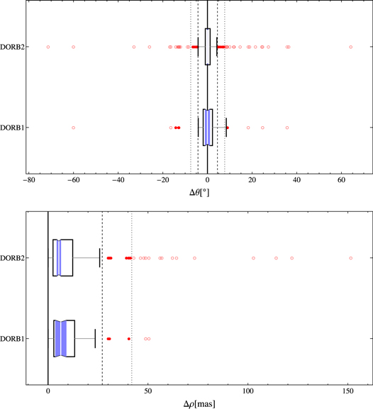
Figure 1. Box plots of residuals obtained from DORB1 and DORB2 for θ (above) and ρ (below). A thick white vertical bar indicates the median, whereas its confidence interval is shown in blue. The vertical boundaries (or hinges) indicate the interquartile range (IQR). Thick line extensions (or whiskers) were, as usual, set at 1.5 × IQR above and below the 25% and 75% quartiles. The notches on the sides of the box were set at ±1.58 × IQR/ , representing the standard deviation of the median if the distribution were normal. Suspected mild outliers are shown as filled red disks and extreme outliers as empty red disks.
Download figure:
Standard image High-resolution imageThe set of potential outliers was carefully analyzed to avoid the deletion of points with significant information. In this way, the modified Thompsonʼs τ technique (Thompson 1935), an objective statistical method for deciding whether to keep or discard suspected outliers in a sample of a single variable, was applied to the residuals for each coordinate. According to ISO 5725-2 (1994), statistically significant outliers at the 99% confidence level were rejected after concluding that none of them might represent genuine values of each population. Thus, 11 outliers were detected in residuals of θ and 8 in residuals of ρ. Results for descriptive statistical parameters are listed in Table 1 and scatterplots of residuals for each coordinate are shown in Figure 2.
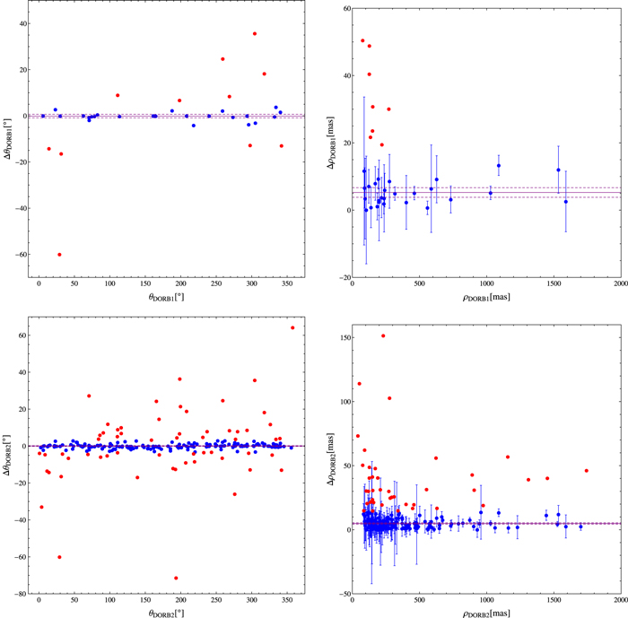
Figure 2. Scatterplots of residuals in each polar coordinate, θ (left) and ρ (right), for the DORB1 (above) and DORB2 (below) data sets. Normal values are indicated with blue circles and outliers with red circles. Vertical bars on the ρ plot show standard uncertainties given by Hipparcos. Solid purple lines show the mean value for each coordinate, whereas dashed purple lines show the upper and lower 95% confidence limits without taking outliers into account. Values at the x-axis have been truncated at 2000 mas since there are only 6 points of 214 between 2000 and 19,000 mas.
Download figure:
Standard image High-resolution imageTable 1. Residuals in Polar Coordinates: Descriptive Statistical Data
| DORB1 |

|

|
| N (points) | 35 | 35 |
| Median | −0.03 | 6.4 |
| MedianCI95% | {−0.32, 0.04} | {3.7, 9.2} |
| Mean | −0.5 ± 4.9 | 11.6 ± 4.6 |
| MeanCI95% | {−5.4, 4.4} | {7.0, 16.3} |
| Wt. mean | ... | 6.3 ± 2.5 |
| Trimean | −0.1 | 9.9 |
| rms | 14.0 | 17.7 |
| DORB1 Without Outliers (at 99%) | ||
| N (points) | 24 | 27 |
| Median | −0.04 | 4.9 |
| MedianCI95% | {−0.32, 0.02} | {2.9, 6.6} |
| Mean | −0.1 ± 0.8 | 5.2 ± 1.4 |
| MeanCI95% | {−0.9, 0.7} | {3.8, 6.7} |
| Wt. mean | ... | 4.9 ± 1.4 |
| Trimean | −0.2 | 5.2 |
| rms | 1.8 | 6.3 |
| DORB2 | ||
| N (points) | 214 | 214 |
| Median | 0.03 | 5.4 |
| MedianCI95% | {−0.06, 0.15} | {4.8, 6.5} |
| Mean | 0.2 ± 1.4 | 12.4 ± 2.7 |
| MeanCI95% | {−1.2, 1.6} | {9.7, 15.1} |
| Wt. mean | ... | 7.6 ± 1.5 |
| Trimean | 0.2 | 9.9 |
| rms | 10.6 | 23.8 |
| DORB2 Without Outliers (at 99%) | ||
| N (points) | 155 | 170 |
| Median | 0.03 | 4.1 |
| MedianCI95% | {−0.05, 0.12} | {3.4, 4.9} |
| Mean | 0.0 ± 0.2 | 4.9 ± 0.6 |
| MeanCI95% | {−0.2, 0.2} | {4.4, 5.5} |
| Wt. mean | ... | 4.3 ± 0.5 |
| Trimean | 0.1 | 4.7 |
| rms | 1.2 | 6.1 |
Download table as: ASCIITypeset image
3.2. Accuracy in θ and ρ
It is widely accepted that the median constitutes a reliable measure of the central location of a univariate data set, the major advantage of this being that compared with the mean, the former is not affected by extreme scores. In any case, a remarkable conclusion can be derived from analysis of the means or, alternatively, from the medians of each coordinate. Residuals in the θ population show mean and median values of nearly zero; in fact, the 95% confidence interval for the mean is symmetrically distributed around zero, including both values.
On the contrary, residuals in ρ present a significant trend of being positive. Note that the confidence interval for the mean does not include the zero at the 95% level, as well as there not being any negative residual in the entire population, the minimum value being +0.03 mas. In fact, we have tested the null hypothesis that the mean of the residuals in ρ is equal to zero ( ) using, as usual, the one-sample Studentʼs t-test. We took the one-sided alternative hypothesis that
  . The result was that the null hypothesis can be rejected at the
  significance level if we remove suspected outliers (
 if we include them). This shows that the Hipparcos angular separations are statistically significantly larger than the reference values with a probability higher than 99.999999%.
Indeed, after removing suspected outliers, the mean bias can be estimated with a relatively high precision at 5.2 ± 1.4 mas (11.6 ± 4.6 mas if we include them), indicating that Hipparcos measurements of angular separations are somewhat larger than those considered to be the most probable values. Even when we calculate the weighted mean (considering standard uncertainties given by Hipparcos), we obtain 4.9 ± 1.4 mas if we remove outliers (6.3 ± 2.5 mas if we include them).
We must note that the origin of these large residuals could be due to complications that arise when deriving the Hipparcos angular separations between double star components. Although a detailed description of the methodology by which the Hipparcos data are obtained is outside the scope of this paper, we must take into account that this procedure is particularly complex for binary stars in comparison with single stars. Many observations have to be performed to obtain the angular separation together with the position angle and the magnitude difference. In addition, systems with separations less than 0.28 arcsec have to be handled more carefully. As a result, formal errors of the double star parameters become functions of both separation and magnitude difference between the components (van Leeuwen 2007b). This could possibly explain the accumulation of outliers below 0.3 arcsec for DORB1 (see the upper right side of Figure 2). It means that this region gathers 8 outliers of 23 values (35%) below that threshold, in contrast with 0 of 12 (0%) above. A similar result is obtained for DORB2, where there are 29 outliers of 116 values (25%) below that in contrast with 15 of 98 (15%) above.
3.3. Precision in θ and ρ
As is normal in these cases, considering the rms as a meaningful measure of the uncertainty of the DHIP observations with respect to those of the DORB1, we conclude that the mean uncertainties in θ and ρ for the Hipparcos observations are actually 18 and 6.3 mas, respectively.
Conclusions reached in Sections 3.2 and 3.3 may be corroborated by taking into account the larger DORB2. Again, very similar results are obtained. These are also listed in Table 1 whereas scatterplots of residuals for each coordinate are shown in Figure 2. In this case we must note that the null hypothesis  (
( being the alternative hypothesis) can be rejected at the
  significance level.
3.4. Hypothetical Correlations
On the other hand, in order to investigate eventual correlations between coordinates and residuals as well as between those and parallaxes, masses, and apparent magnitudes, we have considered the enlarged data set, DORB2.
First, we looked for supposed correlations between residuals of polar coordinates and polar coordinates themselves. However, no significant correlation was found beyond the expected trend of residuals of θ and ρ increasing as ρ decreases (see the bottom part of Figure 3). This effect, more noticeable with the position angles, is probably due to limitations caused by observing systems with angular separations close to the diffraction limit of the instrument.
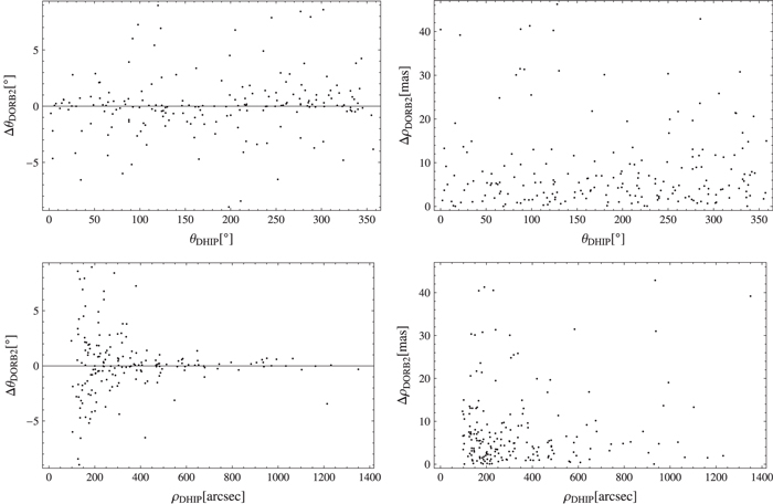
Figure 3. Scatterplots of residuals in each polar coordinate, θ (left) and ρ (right), for the DORB2 data set vs. position angle, θ (above), and angular separation, ρ (below). Both axes have been truncated so that large values are not plotted.
Download figure:
Standard image High-resolution imageRegarding these and other hypothetical correlations between residuals of the coordinates and parallaxes, masses, and magnitudes, we have applied two well-known non-parametric hypothesis tests developed to detect nonlinear relationships: the Kendall τ rank correlation coefficient and the Spearman ρ rank correlation coefficient (Feigelson & Babu 2012). Both tests do not allow for the existence of statistically significant correlations in any of the investigated cases in this subsection. Scatterplots are shown in Figure 4.

Figure 4. Scatterplots of residuals in each polar coordinate, θ (left) and ρ (right), for the DORB2 data set vs. Hipparcos parallax,  (first row), total mass, M (second row), total magnitude, mt (third row), and difference in magnitudes between components,
  –
– (last row). Both axes have been truncated so that large values are not plotted.
Download figure:
Standard image High-resolution image4. HIPPARCOS PARALLAX ACCURACY
Regarding the accuracy of the Hipparcos parallaxes, we carried out a statistical study to check its correlation with the orbital parallaxes obtained from the very accurate data set of visual–spectroscopic orbital elements of the six SB2 systems of the DORB1-SB2 using

where the numerical constant results from expressing  in the same units as a (usually mas), P in days, and KA and KB in km s−1. As usual, to obtain its combined uncertainty,
  , we have propagated uncertainties through a linearized model using the Taylor series.
The aforementioned task was accomplished using three least-squares regression models to estimate the fitted calibration line, in this case, the linear relationship between the dependent variable,  , and the independent variable,
  . The first two are the well-known ordinary least-squares (OLS) and the weighted least-squares (WLS) methods. The last is an errors-in-variables model which, in its most general form (Feigelson & Babu 2012), can be expressed as
with  and
and  being the parallaxes obtained from the orbit and from Hipparcos, respectively, and
  and
and  the corresponding unobserved true parallaxes. On the other hand, a is the intercept and b is the slope of the linear model, and (
 , μ, and η) are the scatter terms. As usual, we made the standard assumption that these are normally distributed with different variances. In addition, considering that the scatter is dominated by heteroscedastic measurement errors in both
  and
and  (for i measurements), we have
  ,
,  , and
, and  . In this bivariate situation, the data are of the form (
 ,
,  ;
;  ,
,  ).
).
In particular, we used a robust errors-in-variables model derived by York (2004), suitable when both variables are subject to heteroscedastic measurement uncertainties that fit the best (optimum) straight line (BSL) to data points with normally distributed uncertainties.
Initially, we considered only Hipparcos parallaxes obtained from the global re-reduction of the Hipparcos data (van Leeuwen 2007a) but we quickly became aware that the old reduction (ESA 1997) showed a best fit. This discrepancy is essentially due to the discordant value of the trigonometric parallax obtained in the new reduction for the HIP 12390 star in comparison with the value obtained not only in the old reduction but also with that calculated from an accurate orbit (Docobo & Andrade 2013). In fact, we suspect that the new trigonometric parallax may have been miscalculated. Therefore we took into account trigonometric parallaxes obtained from both reductions as illustrated in Table 2.
Table 2. Orbital (DORB1-SB2) and Hipparcos (DHIP: 1997 and 2007 Reductions) Parallaxes
| WDS | HIP |
 (mas) (mas) |
 (mas) (mas) |
 (mas) (mas) |
ref |
| 02396–1152 | 12390 | 35.1 ± 1.0 | 36.99 ± 1.76 | 46.55 ± 2.53 | 1 |
| 07518–1354 | 38382 | 63.4 ± 2.4 | 59.98 ± 0.95 | 60.59 ± 0.59 | 2 |
| 15232+3017 | 75312 | 54.62 ± 0.82 | 53.70 ± 1.24 | 55.98 ± 0.78 | 3 |
| 18055+0230 | 88601 | 192.0 ± 4.4 | 196.62 ± 1.38 | 196.72 ± 0.83 | 4 |
| 19311+5835 | 95995 | 58.9 ± 2.0 | 59.84 ± 0.64 | 58.96 ± 0.65 | 5 |
| 21145+1000 | 104858 | 54.89 ± 0.50 | 54.11 ± 0.85 | 54.09 ± 0.66 | 6 |
Note. The WDS identifier, Hipparcos number, and reference of the definitive visual orbit are shown in the first column for each star.
References. (1) Docobo & Andrade 2013, (2) Tokovinin 2012, (3) Muterspaugh et al. 2010, (4) Eggenberger et al. 2008, (5) Farrington et al. 2010, (6) Muterspaugh et al. 2008.
Download table as: ASCIITypeset image
Parameters obtained from the cited models are summarized in Table 3. We list the intercept, a, and the slope, b, along with standard uncertainties, u(a) and u(b). In addition, the 95% confidence intervals for each parameter as well as the coefficient of determination, R2, are also shown. With respect to the latter, a computation of the statistical significance of its square root, the so-called correlation coefficient (r), by means of a two-sided Studentʼs t-test with the null hypothesis that r = 0 and the alternative hypothesis that  shows that the null hypothesis can be rejected at the 10−5 significance level. Scatterplots with linear fits are illustrated in Figure 5.

Figure 5. Scatterplot of Hipparcos (left: ESA 1997, right: van Leeuwen 2007a) vs. orbital parallaxes for the six SB2 stars with definitive visual orbits and doubled-line spectroscopic orbits (in blue). Heteroscedastic measurement uncertainties in both variables are shown. Three least-squares linear fits are plotted: ordinary least squares (blue dotted), weighted fit using only  standard uncertainties (green dashed), and robust best straight line fit considering standard uncertainties in both variables (red solid).
Download figure:
Standard image High-resolution imageTable 3. Parameters for the Least-squares Fits (OLS: Ordinary Least Squares; WLS: Weighted Least Squares; and BSL: Best Straight Line) of Hipparcos and Orbital Parallaxes for the Six SB2 Stars with Definitive Visual Orbits and Doubled-line Spectroscopic Orbits
| a | u(a) | CI95% (a) | b | u(b) | CI 95% (b) | R2 | |
| OLS | 1.89 | 4.13 | {−9.57, 13.35} | 1.01 | 0.04 | {0.88, 1.13} | 0.99222 |
| WLS | −2.62 | 2.10 | {−8.46, 3.22} | 1.04 | 0.02 | {0.97, 1.10} | 0.98961 |
| BSL | 0.40 | 4.38 | {−11.75, 12.56} | 1.00 | 0.07 | {0.80, 1.20} | 0.99530 |
Download table as: ASCIITypeset image
In order to validate Hipparcos measurements of the parallaxes of binary systems, we compared them with those obtained from an accurate computation of the orbital parallax for the DORB1-SB2. The statistical procedure used to perform this takes into account that if both methods lead to the same results the dependence of  on
on  is linear (
 ) with zero intercept (a = 0) and unit slope (b = 1). In our case, we had to consider the parameters a and b and the 95% confidence intervals of both. Scatterplots with the BSL fits and the corresponding 95% confidence intervals for both reductions are shown in Figure 6. Because the confidence interval for a includes zero, it follows that the intercept is not significantly different from zero. On the other hand, since the confidence interval for b includes one, the slope cannot be considered significantly different from one.
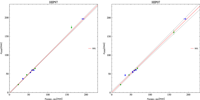
Figure 6. Scatterplot of Hipparcos (left: ESA 1997, right: van Leeuwen 2007a) vs. orbital parallaxes for the six SB2 stars with definitive visual orbits and doubled-line spectroscopic orbits, indicated by blue circles. Heteroscedastic measurement uncertainties in both variables are shown. The robust best straight line (BSL) fit is indicated with a red solid line, whereas dotted lines indicate pointwise 95% confidence intervals. Five independent SB2 stars with definitive visual orbits but without known standard uncertainties in the orbital elements (not used to compute the BSL fit) are indicated with green circles.
Download figure:
Standard image High-resolution imageIn addition, we performed a more rigorous simultaneous test of a composite hypothesis considering the null hypothesis H0: a = 0 and b = 1 against the alternative HA:  and
and  , in both cases (HIP97 and HIP07) using the Fisher–Snedecor distribution for the parameters obtained using the three methods. As usual, the 0.05 level of significance was considered to be a criterion. We found that the null hypothesis cannot be rejected at the 95% confidence level in any case. In fact, it only can be rejected at the 0.64 significance level, this large value indicating a very small significance, that is, that the data provide no evidence that the null hypothesis is false.
Indeed, we can observe (see Figure 7) that the 95% confidence ellipse obtained even using the less robust OLS method contains the ideal point  for intercept and slope, respectively, showing that the DORB1-SB2 reference data set and DHIP07 are not significantly different at the 95% confidence level.

Figure 7. Construction of the 95% confidence ellipse corresponding to the joint test of slope, b, and intercept, a, for the fitted calibration line of parallaxes for the DORB1-SB2 and DHIP07 data sets using OLS (blue). The ideal point  is indicated with a small red disk.
Download figure:
Standard image High-resolution image
With the aim of comparing both reductions, HIP97 and HIP07, we performed an analysis of the residuals of their differences,  and
and  . Descriptive statistical data are summarized in Table 4. From a visual inspection, we can see that means and medians of both sets are compatible with zero at the 95% confidence level. Note that the trimean, calculated using the central three points and recommended for very small data sets (
 ), is also very similar to them.
Table 4. Residuals in Parallax Differences: Descriptive Statistical Data
 (mas) (mas) |
 (mas) (mas) |
|
| N (points) | 6 | 6 |
| Maximum | 4.62 | 11.45 |
| Minimum | −3.42 | −2.81 |
| Median | 0.08 | 2.21 |
| MedianCI95% | {−0.92, 1.89} | {−0.80, 4.72} |
| Mean | 0.39 ± 2.89 | 2.83 ± 5.41 |
| MeanCI95% | {−2.51, 3.28} | {−2.58, 8.24} |
| Wt. mean | −0.39 ± 1.82 | 1.28 ± 4.37 |
| Trimean | 0.44 | 2.40 |
| rms | 2.55 | 5.49 |
Download table as: ASCIITypeset image
Thus, we can conclude that parallaxes obtained by Hipparcos, independent of the reduction considered, do not differ from those obtained using the method of orbital parallaxes applied to binaries with the most accurate orbits. This result is also corroborated by comparison of the BSL fit with five independent SB2 systems with definitive visual orbits but without known standard uncertainties in the orbital elements (not used to compute the BSL fit) as shown in Figure 6.
5. CONCLUSIONS
We have analyzed the 35 binary systems with orbital elements whose positions, have also been measured by Hipparcos. Using robust statistical techniques, we have been able to calculate accuracy and precision both in position angles (θ) and angular separations (ρ). Furthermore, we have selected the six binaries identified as SB2 systems from that trustworthy set whose orbital parallaxes are the most accurate ever calculated. In order to evaluate the accuracy of the Hipparcos parallaxes of binary systems, we have used those binaries as a calibration tool, carrying out several statistical analyses including fits that use robust errors-in-variables models suitable for bivariate heteroscedastic data as well as hypothesis tests.
Our main conclusions follow.
- 1.There is sufficient evidence at the 10−8 significance level to support the claim that angular separations, ρ, measured by Hipparcos in binary systems are systematically overestimated by not less than 5 mas (precisely, 5.2 ± 1.4 mas). This bias is not observed, however, in position angles, θ.
- 2.On the other hand, uncertainties in θ and ρ for the Hipparcos measurements of binary systems are 18 and 6.3 mas, respectively.
- 3.Although there is not a significant correlation between polar coordinates and residuals, an explainable increment of residuals at low angular separations has been found mainly in angular positions. Such an effect probably arises as a consequence of observations carried out close to the diffraction limit of the instrument.
- 4.No statistically significant correlations were detected between residuals in polar coordinates and parallaxes, masses, or apparent magnitudes.
- 5.Regarding parallax calibrations, we concluded that Hipparcos trigonometric parallaxes of binary systems are fully compatible with those obtained from the most accurate visual and spectroscopic orbital elements.
For this research, the authors made use of The Hipparcos Catalog from the European Space Agency (ESA), the Washington Double Star Catalog maintained at the U.S. Naval Observatory (USNO), and the SIMBAD database operated at CDS (Strasbourg, France). This paper was supported by the Spanish "Ministerio de Economía y Competitividad" under Project AYA 2011–26429 as well as by the IEMath–Galicia Network (FERDER–Xunta de Galicia).