


ABSTRACT
We use images acquired by the Cassini Imaging Science Subsystem (ISS) to investigate the temporal variation of the brightness and height of the south polar plume of Enceladus. The plume's brightness peaks around the moon's apoapse, but with no systematic variation in scale height with either plume brightness or Enceladus' orbital position. We compare our results, both alone and supplemented with Cassini near-infrared observations, with predictions obtained from models in which tidal stresses are the principal control of the eruptive behavior. There are three main ways of explaining the observations: (1) the activity is controlled by right-lateral strike slip motion; (2) the activity is driven by eccentricity tides with an apparent time delay of about 5 hr; (3) the activity is driven by eccentricity tides plus a 1:1 physical libration with an amplitude of about 0 8 (3.5 km). The second hypothesis might imply either a delayed eruptive response, or a dissipative, viscoelastic interior. The third hypothesis requires a libration amplitude an order of magnitude larger than predicted for a solid Enceladus. While we cannot currently exclude any of these hypotheses, the third, which is plausible for an Enceladus with a subsurface ocean, is testable by using repeat imaging of the moon's surface. A dissipative interior suggests that a regional background heat source should be detectable. The lack of a systematic variation in plume scale height, despite the large variations in plume brightness, is plausibly the result of supersonic flow; the details of the eruption process are yet to be understood.
Export citation and abstract BibTeX RIS
1. INTRODUCTION AND OUTLINE
One of the most important discoveries of the Cassini mission to Saturn has been the identification of geological activity and anomalous thermal emission at the south pole of Enceladus (Porco et al. 2006; Spencer et al. 2006). This activity manifests itself as ∼100 individual geysers (Porco et al. 2014, henceforth Paper 1) that appear, from a distance, to merge into a single plume, determined by Cassini's in situ experiments to consist of salty ice grains (Postberg et al. 2011) and water vapor, laced with organic and nitrogen-bearing compounds (Waite et al. 2009). Tidal heating has been regarded from the outset as the most plausible, ultimate source of the energy driving this activity, though the details have been uncertain. Early suggestions for the mechanisms underlying these phenomena ranged from shear stresses and the near-surface heating they can produce (Nimmo et al. 2007), to the opening/closing of individual cracks, exposing a subsurface body of water (Hurford et al. 2007), both resulting from the diurnal cycling of tidal stresses across the south polar terrain (SPT).
An important observation is the spatial coincidence found between high-resolution, small-spatial-scale thermal "hot spots" collected by the Cassini visible and infrared mapping spectrometer (VIMS) instrument in the vicinity of the south pole on the Baghdad fracture (Blackburn et al. 2012; Goguen et al. 2013) and the surface locations of specific geysers. This correlation has been interpreted as indicating that it is normal, and not shear stresses, controlling the jetting activity and thermal emission arising from the tiger stripe fractures (Porco et al. 2013). This result is presented in full and discussed at length in Paper 1 in the context of a particular eruption mechanism and the interior structure beneath the SPT.
Additional support for the primacy of normal tidal stresses in controlling Enceladus' activity was provided by the discovery that the plume intensity as observed by the Cassini VIMS instrument is time variable and correlated with Enceladus' orbital position (Hedman et al. 2013), as would be generally predicted from the tidal-opening model (Hurford et al. 2007). Given the growing recognition of the importance of normal tidal stresses in controlling Enceladus' activity, it is desirable to further investigate this phenomenon.
The aim of this paper is to carry out an analysis of plume time variability similar to that of Hedman et al. (2013), but instead using images acquired by the Imaging Science Subsystem (ISS) instrument. As we will discuss below, despite the somewhat different characteristics of the ISS data set, the basic conclusion—that the plume shows time variability correlated with orbital position—is the same. However, here we offer a more extensive analysis in that we study not only the brightness but also the height of the plume as a function of Enceladus' orbital position, and investigate in some detail how to reconcile the observations, both VIMS and ISS, with model predictions. To this end, we examine a series of models in which tidal stresses, associated with different aspects of Enceladus' orbit and rotation, control eruptive behavior. Several of these models give satisfactory fits to the observations, but have very different implications for Enceladus as a whole. While we cannot currently distinguish among them, we discuss how future observations could be used to identify which one (if any) is correct.
The rest of the paper is organized as follows. Section 2 describes the observations and data reduction techniques that we used in studying both plume brightness and scale height. Section 3 discusses the tidal stress models employed, and Section 4 discusses how we quantify the goodness of fit of our models. Section 5 presents our results—both the raw observations and a variety of model fits. Section 6 discusses the implications of the various models, and Section 7 provides a summary.
2. OBSERVATIONS AND DATA REDUCTION
The goal of this work is to determine the temporal variability in the scale height and brightness of the plume3 of material erupting from the SPT of Enceladus. What is seen by the Cassini ISS is, of course, sunlight diffracted by the small particles that compose the plume (Porco et al. 2006). Since the plume is optically thin at visible wavelengths, the integrated brightness measured in ISS images is proportional to the total surface area of lofted ice grains, a good proxy for total plume mass and therefore activity, so long as the average particle size distribution of the plume stays constant regardless of the total amount of mass in it.
The images selected for this study range between 150° and 165° in solar phase angle and lower than |10°| in sub-spacecraft latitude. They vary widely in sub-spacecraft longitude on Enceladus, and in Enceladus' mean anomaly. Their image scales range from 1.9 to 9 km pixel−1 (see Table 1). We found that images with scales much smaller than ∼2 km pixel−1, and therefore higher resolution, did not have a sufficiently large field of view to capture the entire plume and so were not used in this study (see below).
Table 1. The Relevant Parameters for the Images Used, and for the Measurements Reported, in This Work
| Image Number | Mean Anomaly | Raw Int. I/F | Corr. Int. I/F | Total I/F Error | Res. | Original Phase | Sub S/C Lat | Sub S/C Lon | Rev | Date | Scale Ht. | Scale Ht. Error |
|---|---|---|---|---|---|---|---|---|---|---|---|---|
| (°) | (km2) | (km2) | (km2) | (km pixel−1) | (°) | (°) | (°) | (km) | (km) | |||
| N1652824635 | 1.00 | 11.79 | 10.77 | 1.49 | 1.93 | 159.1 | 0.22 | 125.09 | 131 | 2010–137 | 118.3 | 5.4 |
| N1646188916 | 9.38 | 16.05 | 22.59 | 2.73 | 4.30 | 153.5 | 0.28 | 152.23 | 127 | 2010–061 | 118.7 | 4.9 |
| N1637420790 | 21.14 | 45.68 | 26.94 | 4.54 | 3.25 | 164.3 | 0.00 | 90.95 | 121 | 2009–324 | 123.3 | 4.1 |
| N1637420842 | 21.29 | 48.45 | 28.70 | 3.45 | 3.25 | 164.3 | 0.00 | 91.06 | 121 | 2009–324 | 124.2 | 3.9 |
| N1608976498 | 37.86 | 124.10 | 65.73 | 7.33 | 4.46 | 165.4 | −8.41 | 29.84 | 98 | 2008–361 | 145.3 | 5.1 |
| N1714610318 | 81.27 | 11.31 | 20.07 | 1.76 | 2.44 | 150.4 | 0.37 | 111.44 | 165 | 2012–122 | 123.4 | 4.0 |
| N1665895088 | 94.67 | 33.83 | 37.52 | 4.34 | 4.01 | 156.6 | −2.19 | 309.28 | 139 | 2010–289 | 128.9 | 4.6 |
| N1516298600 | 100.64 | 23.70 | 42.43 | 3.53 | 5.98 | 150.3 | 0.33 | 93.54 | 20 | 2006–018 | 100.2 | 5.0 |
| N1750772124 | 103.01 | 46.59 | 24.93 | 2.75 | 3.20 | 165.3 | −7.49 | 244.77 | 193 | 2013–175 | 131.1 | 3.6 |
| N1711536167 | 104.80 | 15.13 | 20.81 | 2.09 | 2.06 | 153.9 | 0.43 | 120.61 | 163 | 2012–087 | 128.1 | 5.1 |
| N1616348791 | 106.80 | 84.26 | 48.50 | 6.95 | 3.88 | 164.6 | −5.32 | 130.42 | 106 | 2009–080 | 129.0 | 5.1 |
| N1708454984 | 107.45 | 18.83 | 19.64 | 2.31 | 2.24 | 157.4 | 0.39 | 108.22 | 161 | 2012–051 | 127.4 | 4.7 |
| N1665899841 | 109.11 | 55.09 | 40.87 | 5.17 | 4.01 | 161.7 | −1.98 | 318.51 | 139 | 2010–289 | 122.8 | 3.8 |
| N1750774330 | 109.71 | 39.54 | 25.06 | 2.34 | 3.31 | 163.5 | −5.55 | 251.87 | 193 | 2013–175 | 134.2 | 4.2 |
| N1516320030 | 165.80 | 42.63 | 58.78 | 9.10 | 5.58 | 153.8 | 0.38 | 163.53 | 20 | 2006–018 | 106.9 | 5.8 |
| N1634159832 | 197.86 | 84.75 | 77.69 | 6.13 | 2.58 | 159 | −0.28 | 292.39 | 119 | 2009–286 | 127.6 | 4.8 |
| N1634162091 | 204.71 | 105.97 | 80.02 | 6.29 | 2.57 | 161.5 | −0.28 | 296.82 | 119 | 2009–286 | 130.3 | 4.3 |
| N1634163141 | 207.92 | 113.58 | 77.27 | 6.78 | 2.56 | 162.7 | −0.29 | 298.78 | 119 | 2009–286 | 131.1 | 4.7 |
| N1651010460 | 251.73 | 72.71 | 53.15 | 5.37 | 5.96 | 161.9 | 0.02 | 47.13 | 130 | 2010–116 | 127.8 | 5.5 |
| N1643187583 | 253.99 | 53.86 | 62.73 | 5.78 | 5.73 | 156 | −3.79 | 24.36 | 125 | 2010–026 | 118.9 | 5.7 |
| N1643192383 | 268.58 | 61.70 | 48.46 | 4.89 | 5.38 | 161 | −3.88 | 33.98 | 125 | 2010–026 | 123.6 | 5.7 |
| N1640477223 | 302.93 | 31.14 | 25.17 | 2.93 | 3.28 | 160.6 | −2.92 | 20.27 | 123 | 2009–359 | 128.8 | 5.3 |
| N1646167283 | 303.68 | 14.12 | 17.65 | 2.55 | 6.34 | 155.1 | 0.21 | 84.87 | 127 | 2010–060 | 120.1 | 6.4 |
| N1640478423 | 306.58 | 27.00 | 27.84 | 2.98 | 3.20 | 157.6 | −2.85 | 20.84 | 123 | 2009–359 | 130.9 | 6.0 |
| N1516367311 | 309.51 | 24.46 | 29.22 | 6.51 | 9.28 | 155.7 | 0.24 | 310.27 | 20 | 2006–019 | ||
| N1646170883 | 314.62 | 10.09 | 11.72 | 1.78 | 5.97 | 156.1 | 0.22 | 94.86 | 127 | 2010–060 | 107.2 | 4.3 |
| N1646174483 | 325.55 | 11.37 | 12.64 | 1.91 | 5.59 | 156.6 | 0.23 | 105.26 | 127 | 2010–060 | 116.3 | 6.2 |
| N1660401826 | 332.44 | 13.78 | 9.85 | 1.68 | 1.88 | 162.1 | −6.69 | 126.14 | 136 | 2010–225 | 140.0 | 6.4 |
| N1646179299 | 340.17 | 13.42 | 14.95 | 1.49 | 5.11 | 156.6 | 0.24 | 119.91 | 127 | 2010–060 | 125.3 | 5.0 |
| N1639068152 | 343.91 | 34.78 | 18.58 | 4.24 | 3.91 | 165.4 | −0.02 | 60.83 | 122 | 2009–343 | 128.1 | 7.2 |
| N1646182899 | 351.10 | 13.83 | 16.23 | 1.56 | 4.78 | 155.9 | 0.26 | 131.51 | 127 | 2010–061 | 122.0 | 5.5 |
Notes. Raw Int. I/F is the integrated I/F derived in the manner described in the text; Corr. Int. I/F is the integrated I/F corrected, using the phase function shown in Figure 4, to a phase angle of 158°. Total I/F error is the sum of all the estimated errors derived for the final value of integrated I/F and the error that is shown for each datum in Figure 9 in the main text. Res. is the image scale of the image in km pixel−1. Sub S/C Lat and Sub S/C Lon are the latitude and west longitude on Enceladus of the sub-spacecraft point. Rev is the orbit number of the Cassini trajectory around Saturn. Scale Ht. is the scale height derived as described in the text. The other columns are self-explanatory.
Download table as: ASCIITypeset image
Each image was calibrated and flat-fielded using the ISS calibration software CISSCAL, version 3.7, and then pointing corrected. Details of the steps involved in the reduction of images, subtraction of the E ring, and the subsequent calculations to produce an absolute integrated brightness and a scale height for the plume as observed in each image are given below. In brief, to determine the plume's brightness, a rectangular region of integration was selected, extending vertically from 100 km to 500 km above the south pole, and horizontally across the breadth of the image. Then, at each horizontal position in this rectangle, the vertical integral ∫(I/F)dy was obtained, where I/F is the absolute brightness and dy is the distance in kilometers on the sky at each altitude. These vertically integrated values were then plotted to produce a horizontal scan across the image. After subtracting out the remaining background, the area under the curve in the scan from each image was calculated to arrive at the final integrated I/F = ∫∫(I/F) dy dx.
The data reduction and computations for determination of the plume scale heights were similar, though different in some important regards, which are discussed in detail below.
Because the images were taken over a large range in solar phase angles, variations in plume brightness due simply to angular variation in particle scattering efficiency are present. To remove these geometry-dependent brightness variations, the integrated I/F's had to be normalized to the same phase angle. This required determining the phase function of the plume particles, which in turn requires knowing the particle size distribution. In the end, all integrated I/F's were corrected to 158° phase in a process described below.
2.1. Data Reduction Details
An original, unprocessed image of the southern limb of Enceladus that is representative of the kind used in this work is shown in Figure 1(a). The field of view of the narrow angle camera was deliberately placed to avoid the bright crescent of the moon in these high phase images and the stray light that it can introduce into the optics. Once such images are flat-fielded and photometrically calibrated (Porco et al. 2004; West et al. 2010), the next steps in the image reduction involve correcting for the pointing uncertainty and subtracting out any background in the image due to other sources of light, such as the E ring.

Figure 1. (a) Image N1634163141 taken in the clear filter. (b) Image N1634163141, calibrated, cleaned of bright pixels, and background (dark current and E ring) removed, showing in green the rectangular area (400 km tall) in which the I/F values were integrated.
Download figure:
Standard image High-resolution imagePointing correction. In order to assign accurate planetocentric coordinates to any pixel falling either on the surface of Enceladus or in the sky plane, the three-dimensional locations of the spacecraft and the moon as well as the orientations in space of the moon and the camera at the time the image is taken must be known accurately. The first three items are supplied by JPL in files called kernels. The target-relative location and orientation of the camera and its field of view, respectively, however, must be calculated for each image using the process of image navigation.
For this work, the observed locations in the image of the points forming the limb of Enceladus serve as a set of fiducials for aligning the expected and observed position of the moon. For all the images used here, the sunlit limb of Enceladus was the fiducial; in some of the images where it was visible, the Saturn-lit limb was used. Points on the limb coincident with the plume's location were excluded from the fit; those near the horn of the sunlit crescent were often excluded, as the back lighting by the E ring would confuse the algorithm. All these points were extracted algorithmically: i.e., by calculating the radial brightness gradient near the edge of Enceladus's disk and selecting the half-power point. The extracted points were then compared to the expected positions of the limb computed from the reconstructed spacecraft trajectory and camera orientation; the difference between the two is the correction to the camera pointing and its orientation that is then applied to all pixels in the image. The final result is a "navigated" image of the moon on which has been projected an accurate coordinate system. All measurements used in this work have been made on navigated images (see Table 1).
E ring removal. Despite the calibration process which removes dark current from the images and applies a flat-field correction, the background in the image is bright and not uniform because of Enceladus' apparent position within the E ring. It also varies from image to image because of the differing longitudes from which the images were taken. To ensure accurate plume photometry, this background had to be removed.
We begin the removal process by taking from each image a series of contiguous scans, 16 pixels wide and extending the entire length of the image, each contacting but not overlapping the next, oriented parallel to the E ring. The region near Enceladus and the plume, as well as points that were corrupted by stars, cosmic rays, or in rare cases Saturn or its rings, were excluded. As the background brightness generally has some slight curvature to it, we performed a quadratic fit to each scan which resulted in a noise-free background I/F, filling in the region under Enceladus and the plume as well. We then combined all the fits to produce a synthetic image of the E ring background. This synthetic product was then subtracted from the original calibrated image; cosmic rays and stars were filtered out at this stage using a simple median filter with a 5 × 5 window.
Figure 1(b) shows the contrast-enhanced version of the same image in which the background, including the E ring, was removed as described above. Our 400 km tall integration region for determination of the integrated plume brightness is also shown.
At each horizontal position within the integration region shown in Figure 1(b), the vertical integral ∫(I/F)dy was obtained, where I/F is the absolute brightness and dy is the distance in kilometers on the sky at each altitude. These vertically integrated values were then plotted to produce a horizontal scan across the image, showing a peak centered on the plume. The final integrated I/F, ∫∫(I/F) dy dx, is given by the "area under the curve" shown in Figure 2, bounded on the bottom by the background light that is subtracted out in this last computation. As the navigation error is believed to be no more than ±1 pixel, we estimated the variation in the final integrated I/F due to navigation errors by varying the estimated position of the Enceladus limb by 1 pixel and deriving the corresponding integrated I/F.
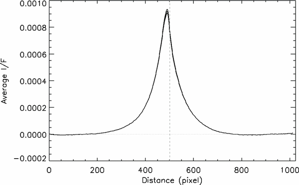
Figure 2. Horizontal scan of vertically integrated (I/F)dy values, as described above, taken from Figure 1(b), and averaged. Three averaged scans are shown, each corresponding to a shift of 1 pixel in the position of the Enceladus limb, as a check on the navigation uncertainty. The horizontal dotted line shows the lower boundary on the region within which the values were summed to derive a final area-under-the-curve result.
Download figure:
Standard image High-resolution imagePhase angle correction. To compute the phase function for the particles in our integration region, we took the mass distributions obtained for the Enceladus plume by the Cassini VIMS instrument for particle sizes from 1 to 4 μm (Figure 4 of Hedman et al. 2009), turned them into size distributions, and linearly extrapolated the logarithm of the results at 1 and 2 μm into the visible range of the spectrum, down to 0.1 μm, where the ISS sees. This was done for the three VIMS cubes and four altitudes between 100 km and 240 km (Hedman et al. 2009) that overlapped our integration region, resulting in 12 different size distributions from 0.1 μm to 3 μm. (We did not choose the data from the highest altitudes, as these were the most unreliable in the VIMS data.) To each of these we fit a power law; averaging the coefficients obtained for each size distribution in this way yielded an average power law exponent q = 2.93 ± 0.18. These results are shown in Figure 3.

Figure 3. Twelve size distributions, along with our fitted average (solid line), obtained from three VIMS cubes of the Enceladus plume taken over the course of ∼4 hr. The values at 1 μm and 2 μm are directly from Hedman et al. (2009); the value at 0.1 μm is logarithmically extrapolated from the values at 1 and 2 μm. We plot the 3 μm value as well.
Download figure:
Standard image High-resolution image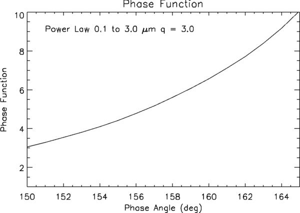
Figure 4. Phase function P(α) of the plume particles at altitudes between 100 km and 500 km derived using the Mie scattering code of Mischenko et al. (2002) and the particle size distribution shown in Figure 3.
Download figure:
Standard image High-resolution imageThis averaged size distribution was then used as an input to a publicly available Mie light-scattering code (Mischenko et al. 2002) to determine the expected brightness variation of the plume as a function of phase angle α. For this work, only the relative difference in brightness, and not the absolute brightness, was required. As our power law coefficient was statistically indistinguishable from three, we used the standard power law distribution with a coefficient of three, a minimum radius of 0.1 μm, and a maximum radius of 3 μm. The resulting phase function P(α) was indistinguishable in the region between 150° and 165° phase angle from that derived by Ingersoll & Ewald (2011) using very high phase ISS images of the Enceladus plume. The phase function produced, shown in Figure 4, was then used to modify the integrated I/Fs to the value they would have if the images were all taken at the same phase angle: I/Fnew = I/Fold*(P(αnew)/P(αold)). The phase angle chosen for this correction was α = 158°, which lies in the middle of the range of phase angles spanned by the observations.
Photometric uncertainty. The uncertainty assigned to the final integrated I/F for each image arises from several possible sources: navigation, photon statistics, uncertainty in the phase angle correction described above, and systematic photometric uncertainties.
The contribution as described above from navigation was found to be negligible. The uncertainty in the correction of the integrated I/F to a common phase angle arises because of an uncertainty in the true phase function of the particles. This is difficult to quantify but we take as significant the fact that we used particle size distribution data from the Cassini VIMS instrument to determine the form of our phase function and in the end, our results agreed almost perfectly with the results of another group using a different ISS data set. We consequently have assumed that errors in this process are small and likely to be swamped by other sources. The uncertainty due to photon statistics can be directly estimated from the average brightness. And, as it is widely believed that one cannot do any absolute astronomical photometric measurement better than about 5%–10%, we have assigned a systematic uncertainty to our data of 7%. In the end, this last source of uncertainty is the dominant one. The total error is a sum of all of these sources and is given in Table 1.
Resolution dependencies. As the plume is an extended light source, subtracting out the background runs the risk of subtracting part of the plume, as it can be difficult to differentiate it from the background E ring at large distances from Enceladus. This accidental subtraction becomes more likely with higher resolution images, as the plume occupies more of the image at high resolution than low. Indeed, our attention was brought to this issue when we noticed that images with image scales as low as ∼1 km pixel−1 had, in general, lower integrated I/F's, regardless of Enceladus' orbital position.
Figure 5 illustrates the problem. Here, we have taken one image with 4.5 km pixel−1 image scale and calculated scans of vertically integrated I/F across the image in four non-overlapping 100 km tall integration regions instead of one 400 km tall region. On this figure, we have noted the boundaries of hypothetical images having the same view of the plume but higher resolution: i.e., image scales of 3, 2, and 1 km pixel−1. What is immediately clear is that, while the 3 and 2 km pixel−1 "image boundaries" cut all four scans at points where the brightness in the slab has unambiguously leveled out, and can therefore confidently be regarded as background, the same cannot be said for the 1 km pixel−1 boundaries, which cut the scans on the wings of the plume at all four altitudes. The background level determined in such an image would subtract out part of the plume, producing a systematically lower integrated I/F, which is what the reduction of our highest resolution images had in fact indicated.
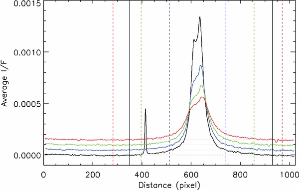
Figure 5. Scans of vertically integrated and averaged I/F's for four non-overlapping horizontal integration regions, each 100 km tall, ranging from 100 km to 500 km altitude above the surface, obtained from a 4.46 km pixel−1 image (N1608976498). The boundaries of the 3, 2, and 1 km pixel−1 hypothetical images are marked by the red, green, and blue vertical dashed lines, respectively. The correspondingly colored dot-dashed lines connecting the vertical lines show where the backgrounds would be calculated for the hypothetical images. The black vertical lines denote the limits that were actually used to compute the 2D integrated I/F tabulated in Table 1.
Download figure:
Standard image High-resolution imageIn extending this resolution analysis to all the images in our data set having image scales ∼4 km pixel−1 and smaller, we found that any variation in the integrated I/F produced by these effects was well accounted for in all cases by our final estimated uncertainties for images having 3 km pixel−1 image scales, was accounted for 2/3 of the time for images with 2 km pixel−1 image scales, but never accounted for in 1 km pixel−1 scale images. Hence, we have limited the highest resolution used in this study to 1.9 km pixel−1.
Enceladus mean anomaly. We determined the mean anomaly of Enceladus at the time of each image by interpolating between the values of the moon's orbital longitude from periapse, or mean anomaly, as determined from orbital integrations and tabulated for the entire Cassini mission in the kernels provided by JPL. The particular kernel used in this work is 110818AP_SCPSE_11175_17265.bsp and contains the ephemerides for the Cassini spacecraft and all the large satellites of Saturn. The Enceladus mean anomalies thus interpolated are given in Table 1.
2.2. Scale Height Determination
Along with the time variability of the two-dimensional (2D)-integrated I/F of the plume, we investigated the variation in scale height of the plume as a function of both the plume's brightness and the orbital position of Enceladus. The reduction of the images for this task was much the same as that outlined above, except in two regards: (1) instead of using a single, 400 km tall horizontal slab as our integration region, we integrated the brightness in concentric azimuthal scans, each keeping a constant radial distance from the surface of the moon, and (2) these scans began at an altitude of 50 km, the highest one extended up to 500 km altitude, each was 50 km tall and 40° wide in azimuth, and all were centered in azimuth on the south pole. A sample image with these scans overlaid is shown in Figure 6(a). For this task it was important to integrate the light that comes from the same altitude; azimuthal scans, though not perfect when comparing images taken from different sub-spacecraft longitudes, were a better choice than horizontal slabs.
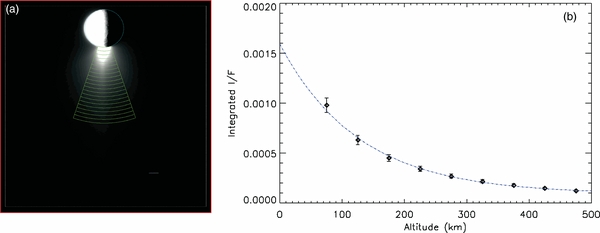
Figure 6. (a) Sample image (N1634159832) showing the series of azimuthal integration regions used in the computation of scale height. The partial shells are each 50 km in altitude and 40° wide azimuthally, centered on the south pole. The image has been brightened to make the plume more visible. (b) The results of integrating the plume brightness within the azimuthal regions shown in panel (a) as a function of altitude. The dash-dot blue line is the fit to an exponential decay plus a constant offset. The scale height for this image is 128 km.
Download figure:
Standard image High-resolution imageWe integrated the I/F in each of these concentric, partial shells to derive an integrated I/F versus altitude. To these reduced data, we fit an exponential function of altitude plus a constant offset and found the scale height from the exponential portion of the fit. Figure 6(b) shows an example of the integrated I/F as a function of altitude as well as the fit to the data.
Figure 7(a) shows the plume scale heights derived from the azimuthal scans for all the images in our data set, plotted versus mean anomaly; these values are also given in Table 1. While there is a lot of scatter in the data, there is clearly no dependence of scale height on mean anomaly. Figure 7(b) is a plot of scale height, this time plotted against integrated plume brightness: again, there is no obvious dependence on the plume brightness. The plume scale height is effectively constant with respect to brightness and mean anomaly. Using horizontal slabs instead of azimuthal scans did not change these conclusions. Their significance is discussed in the Discussion section.
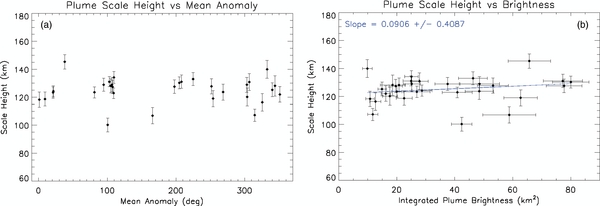
Figure 7. (a) Plume scale height vs. mean anomaly. The scale height does not vary as a function of mean anomaly and is effectively a constant at all orbital positions. (b) Plume scale height vs. plume integrated brightness. As per panel (a), we see no dependence of the scale height on brightness.
Download figure:
Standard image High-resolution image3. TIDAL STRESS MODEL
The tidal model consists of three parts: calculation of the tidal stress tensor as a function of time, resolving the stress tensor onto individual fractures, and calculating the fraction of fractures open.
Tidal stress tensor. To calculate the tidal stress tensor, we followed the method of Appendix A in Hurford et al. (2009) and verified that we could reproduce Figure 5 of Hurford et al. (2009), Figure 2 of Hurford et al. (2007), and Figure 3 of Smith-Konter & Pappalardo (2008). Note that care has to be taken in the longitude convention employed. Note also that this treatment assumes an elastic shell; we briefly discuss the implications of viscoelastic behavior in Section 6. For a case in which obliquity is zero, the instantaneous angular distance θ(t) between a point on the surface (δ, λ) and the tidal bulge is given by
Here δ and λ are latitude and west longitude, e is eccentricity, n is mean motion, F is the amplitude of the 1:1 physical libration, and we have included a possible phase lag ψ. The eccentricity term describes the effect of optical librations (the apparent motion of Saturn in the sky due to the non-circular nature of Enceladus's orbit). We assume that the physical libration term is in phase with the eccentricity term. In the absence of physical librations, we verified that this method yields the same results as that employed by Wahr et al. (2009). We also note that these two methods are equivalent only if the degree-2 Love numbers h2 and l2 used in the approach of Wahr et al. (2009) are in the ratio h2 = 4l2. In Nimmo et al. (2007) it was assumed that h2 = 0.2 and l2 = 0.04; in this work we also take h2 = 0.2, so that the implied value of l2 is 0.05. This explains small differences between the results obtained here and the results of Nimmo et al. (2007). All other elastic and tidal parameters are identical to those employed in Nimmo et al. (2007). Because we are primarily interested in the signs of the stresses (extensional versus compressional), the magnitudes of the calculated stresses are not very important. As a result, uncertainty in parameter values such as the Love numbers are of secondary importance. However, the ratio h2/l2 does affect our results slightly: adopting a lower value of l2 (e.g., the 0.04 value used by Nimmo et al. 2007) results in a slightly smaller apparent phase shift (see below). Our approach assumes a spherically symmetric structure; lateral variations in shell properties may affect the results (see Section 6).
For the case when a resonant libration with a period ratio of 4:1 or 3:1 occurs, we follow Wisdom (2004) and modify the above equation slightly to read
where FM is the amplitude of the M:1 libration. In both the 3:1 and 4:1 models, neighboring orbits will be characterized by different surface stress patterns, and the entire pattern repeats every third or fourth orbit, depending on the resonance. As there is no way to know a priori at which orbit the pattern begins, in each resonance, we shift the pattern one orbit at a time, perform a least-squares fitting analysis, determine the residuals, and then shift the pattern by one orbit and repeat the fitting process. This resulted in three possible solutions for the 1:3 resonance, and four for the 1:4. For each resonance, the orbit shift that gave the smallest minimum residuals has results summarized in Tables 2 and 3 below.
Table 2. Summary of Results of Best-fitting Models
| All ISS data | Degrees of Freedom | a | b | Phase Lag/Libration | Lower Bound | Upper Bound | Min.  |
Min. F12 |
|---|---|---|---|---|---|---|---|---|
| (km2) | (km2) | |||||||
| Constant I/F | ν1 = 29 | 20.6 | ... | ... | ... | ... | 24.0 | ... |
| Phase lag ψ | ν2 = 27 | 7.5 | 56.0 | 62° | 610 |
642 |
12.6 | 1.90 |
| Phase lag ψ* | ν2 = 27 | 12.0 | 53.0 | 64° | 579 |
713 |
11.6 | 2.06 |
| Phase lag ψ + Libration Fl | ν2 = 27 | 12.0 | 38.0 | 49° | n.d. | n.d. | 17.5 | 1.37 |
| Zero phase lag | ν2 = 28 | 15.0 | 32.0 | 0° (fixed) | ... | ... | 20.6 | 1.17 |
| Zero phase lag, strike slip (σmin = 20 kPa) | ν2 = 28 | 9.0 | 71.0 | 0° (fixed) | ... | ... | 16.4 | 1.47 |
| Libration F | ν2 = 27 | 12.0 | 62.0 | 070 |
063 |
077 |
9.94 | 2.41 |
| Libration F (σmin = 20 kPa) | ν2 = 27 | 15.0 | 77.0 | 085 |
054 |
098 |
8.30 | 2.90 |
| 1:3 libration F3 | ν2 = 27 | 12.0 | 42.5 | 150 |
n.d. | n.d. | 15.3 | 1.57 |
| 1:4 libration F4 | ν2 = 27 | 15.0 | 39.5 | 075 |
n.d. | n.d. | 15.7 | 1.53 |
| Rev 098 excluded: | ||||||||
| Constant I/F | ν1 = 28 | 20.6 | ... | ... | ... | ... | 23.6 | ... |
| Phase lag ψ | ν2 = 26 | 7.5 | 56.0 | 62° | 539 |
707 |
11.0 | 2.15 |
| Zero phase lag | ν2 = 27 | 15.0 | 32.0 | 0° (fixed) | ... | ... | 20.1 | 1.17 |
| Libration F | ν2 = 26 | 12.0 | 62.0 | 070 |
062 |
079 |
8.50 | 2.78 |
Notes. The misfit is  ("min." means minimum), a and b are fitting parameters, and F12 is a measure of the statistical significance of this misfit. A large F12 (>1.89 or 1.92, see the text) means that the model is significantly better (at the 95% confidence level) than a model in which I/F is held constant. Upper and lower bounds are calculated by determining where F12 equals the critical value (1.89 or 1.92). "n.d." means "not determined. Note that the shell phase lag is ∼7° smaller than the values of ψ obtained here, owing to the time-of-flight of ejected particles. In obtaining the libration amplitude F, 7° is subtracted from the mean anomaly of each observation prior to fitting, to account for this time-of-flight effect. Results are obtained assuming that each digitized fracture segment (Figure 8) contributes equally to the overall plume flux, except for the case marked *, in which the 98 jet locations identified in Paper 1 were used instead. The three favored models are marked in bold.
Download table as: ASCIITypeset image
Table 3. Summary of Results of Best-fitting Models to VIMS Observations (Hedman et al. 2013)
| VIMS data | Degrees of Freedom | a | b | Phase Lag | Lower Bound | Upper Bound | Min.  |
Min. F12 |
|---|---|---|---|---|---|---|---|---|
| (km) | (km) | |||||||
| Constant CEW | ν1 = 252 | 0.092 | ... | ... | ... | ... | 153 | ... |
| Phase lag ψ | ν2 = 250 | 0.015 | 0.25 | 75° | 0° | 981 |
40.0 | 3.83 |
| Zero phase lag | ν2 = 251 | 0.045 | 0.160 | 0° (fixed) | ... | ... | 62.4 | 2.45 |
| Libration F | ν2 = 250 | 0.045 | 0.228 | 080 |
0° | 135 |
36.3 | 4.21 |
Notes. Notation is as for Table 2, except that we are fitting corrected equivalent width (CEW). Note that a very wide range of phase lags is permitted. Here the critical value of F12 at the 95% level is 1.25.
Download table as: ASCIITypeset image
Enceladus is predicted to experience librations with large amplitudes (Fl ≈ 04) on periods of 5–10 yr owing to mutual interactions with neighboring satellites (Rambaux et al. 2010). These long-period librations do not cause appreciable tidal heating, but will generate stresses: a positive true longitude denotes a situation in which the instantaneous sub-Saturnian point has moved ahead of a fixed point on the surface. In this case, the tiger stripes spend more than half the orbit in tension. Long-period librations are readily modeled by modifying Equation (1): the final term on the right-hand side becomes Fl(t), where the time variability is determined by the different interaction periods (Rambaux et al. 2010).
Resolving the stress tensor. For a particular fracture segment, the instantaneous tidal stresses may be resolved into a normal component σxx and a shear component σxy using the approach outlined in the supplementary online material of Nimmo et al. (2007). Here we are concerned with the opening and closing of segments; we define a segment to be open when σxx > 0. This criterion is strictly correct for shallow regions in which overburden stresses are small (Smith-Konter & Pappalardo 2008). Figures 8(a)–(c) show the mean anomaly at which particular fracture segments first experience opening (σxx > 0), for three different models. Figure 8(d) similarly shows the mean anomaly at which particular fracture segments first experience right-lateral (σxy > 0) stresses.
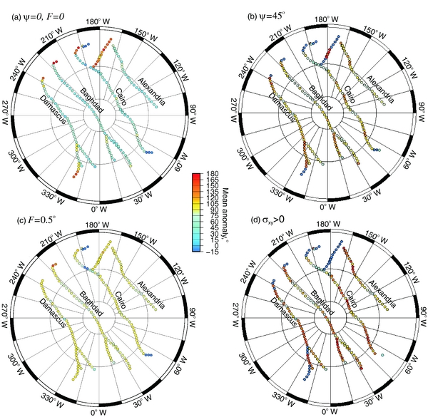
Figure 8. (a) Mean anomaly at which individual fracture segments first experience opening (σxx > 0) in a model with ψ = 0 and F = 0. Polar stereographic projection of region south of 64° S, showing locations of digitized fracture points. Only every third point is shown for clarity (220 points are shown). (b) As for panel (a), but with ψ = 45°. (c) As for panel (a), but with F = 05. (d) As for panel (a), but showing mean anomaly at which individual fracture segments first experience right-lateral shear (σxy > 0).
Download figure:
Standard image High-resolution imageFraction of fractures open. Once the instantaneous normal and shear stresses on each fault segment are known, it is then simple to calculate what fraction of these segments are open (undergoing extensional normal stresses) as a function of time. That fraction f is the prediction that can then be compared with the observed variations in integrated plume brightness. We relate I/F to f as follows:

where a and b are scaling parameters and f depends on either the libration amplitude or the assume phase lag.
In general we assume that each digitized fault segment contributes equally the overall observed plume flux. As a check, we instead assumed that each of the 98 individual jets identified by Paper 1 contributed equally to the flux. As noted in Table 2, this alternative assumption does not yield significantly different results.
4. STATISTICAL ANALYSIS
The χ2 misfit between observation y0 and model ym is calculated as follows:
where σi is the uncertainty associated with the ith observation and there are N observations in total. We define the reduced chi-squared misfit  as
as

where ν is the degrees of freedom (=N – n – 1), where n is the number of parameters to be estimated. In our standard case, n = 3 (the two scaling parameters a and b and one fitting parameter, e.g., the phase lag).
A single tidal stress calculation yields the fraction of the tiger stripes open f as a function of mean anomaly. To compare this result with the observations, we assume that I/F varies linearly with f (Equation (3)). Our model I/F curves also vary with the value of the shell phase lag ψ, forced libration amplitude F, or resonant libration amplitude FM (see above). To find the best-fit set of parameters, we therefore perform a simple grid search in which a, b and (ψ or F or FM) are varied until the minimum  value is obtained.
In the following, we wish to investigate whether our model produces a significant improvement in fit compared to a model in which I/F does not vary with time or orbital position. To do so, we follow the approach of Bevington (1969, p. 196ff.) and compare the  values of the constant I/F model (model 1) with our time-varying models (model 2). By using the F-test we can assess whether the reduction in misfit associated with the time-varying models is statistically significant.
For the constant I/F model, we simply assume I/F = a and solve for the value of a which minimizes the χ2 misfit. This model (model 1) thus has n = 1 while model 2 has n = 3.
For the full data set, ν2 = 27(N = 31, n = 3) and ν1 = 29. For the data set excluding a single anomalous point (rev 098), ν2 = 26 and ν1 = 28. The relevant quantity is the ratio

For the full data set, the value of F12 which is probable at the 5% level is 1.89 while for the reduced data set, the 5% value is 1.92. In other words, values of F12 which are smaller than this value do not yield a significant improvement over the constant I/F case (at the 95% level). Conversely, if a time-dependent model yields an F12 value larger than the critical value, then it is preferred over a constant I/F model.
For each value of phase lag or libration amplitude, we find the values of a and b that minimize the χ2. Doing so allows us to calculate the value of F12 as a function of phase lag/libration amplitude, and thus to determine the 95% confidence limits in the parameter of interest.
5. MODELING RESULTS
Figure 9 is a plot of our data and the results from our tidal modulation models; these results are tabulated in Table 2. Although there is some scatter, the integrated plume brightness data are generally lowest when Enceladus is close to Saturn (mean anomaly M ∼ 0°) and highest at M ∼ 210°. This result is in approximate agreement with the VIMS results (Hedman et al. 2013) and theoretical predictions (Figure 5 of Hurford et al. 2009).

Figure 9. Comparison of observations and model predictions. Numbers indicate Cassini's orbit number (Table 1). The solid lines are based on the fraction of tiger stripes experiencing extensional normal stresses as discussed in Section 3. This fraction f is converted into a predicted I/F by linear scaling: I/F = a + (b − a)f. (a) Simple time-delay model fitted to the ISS data, where a = 7.5 km2 and b = 56 km2. The bold line is the minimum-misfit solution and includes a model phase lag ψ of 62°; the thin line is the same model but without a phase lag (ψ = 0). The thin and bold lines have misfits  of 20.6 and 12.6, respectively. (b) Misfit as a function of ψ, where for each ψ the best-fit values of a and b are also solved for. The shaded region gives the range of ψ at the 95% confidence level (Section 4). The actual phase lag is ∼7° less than ψ because of the time-of-flight of jet particles. (c) As for panel (a), except the model shown is one in which an in-phase forced libration component with amplitude F of 07 is added to the ψ = 0 model and a = 12, b = 62 km2. The mean anomaly of each observation has been reduced by 7° to account for time-of-flight. (d) As for panel (b), but varying the libration amplitude. The minimum misfit is
  = 9.94 and the range of F is 063–077.
Download figure:
Standard image High-resolution imageHowever, our observations diverge from the simple predictions in two ways. First, we observe a background mass flux at all times, even when theory suggests no fractures should be open. Second, there is a mismatch in timing between the observations and the simple theory of tidally modulated crack opening and closing (Hurford et al. 2009). Particles launched on ballistic trajectories will reach a maximum altitude of 250 km (the mid-point of our integration region) after about 40 minutes, corresponding to an angular lag of ∼7°. The timing mismatch that we infer is much larger.
The thin line in Figure 9(a) is based on the simple model and includes a constant background plume flux (a > 0; Section 3). Although the model provides a reasonable match, the observed increase in brightness (M ∼ 90°) and the decrease (M ∼ 270°) both occur at larger mean anomalies (later times) than predicted. As tabulated in Table 2, a significantly improved fit (bold line in Figure 9(a)) can be obtained by introducing a time lag of about 5.7 hr (62° phase lag) to the model. Figure 9(b) shows that model time lags in the range 5.6–5.9 hr (610–642) fit the observations better at the 95% confidence level than a model in which I/F is constant (Table 2). Excluding the anomalous rev 098 point results in an identical best-fit phase lag but in a wider and probably more realistic range of 4.9–6.4 hr (539–707; Table 2). After correcting for the 40 minute ascent time we obtain an apparent time lag of 5.1 ± 0.8 hr.
Table 2 shows that we obtain very similar results if, instead of assuming that all tiger stripe segments contribute equally to the plume flux, we use the 98 jet locations identified in Paper 1. Thus, our results do not depend on the details of the jet locations or tiger stripe geometry.
An alternative way of fitting the observations is shown in Figure 9(c). Here, in addition to the usual eccentricity tides (Hurford et al. 2007), an additional in-phase forced longitudinal libration with an amplitude of 07 (a displacement of 3 km) has been added (Hurford et al. 2009), resulting in a fit slightly better than the time lag model. Such a physical libration is potentially detectable by repeat imaging of surface landmarks. However, theoretical arguments (Rambaux et al. 2010) based on the assumption of a solid Enceladus predict an amplitude of 0026–0032, an order of magnitude smaller than our results. We do not favor models invoking a resonant libration with a period of 1/3 (Wisdom 2004) or 1/4 (Porco et al. 2006) of the orbital period because they both produce poor fits to the data (Table 2), and they are not consistent with the recently measured gravity coefficients (Iess et al. 2014). As the predicted obliquity of Enceladus is very small (Chen & Nimmo 2011), we ignored obliquity tides.
We also investigated whether some of the scatter in the data could be due to the effect of long-period librations. In doing so, it became clear that the Rambaux et al. (2010) analysis contained an error in the assumed reference epoch (B. Noyelles 2013, private communication). After correcting for this error, we found that including the long-period librations significantly reduced the quality of fit when solving for a phase lag (Table 2). This result is surprising, because the long-period librations do not depend on the poorly known interior properties of Enceladus, but only on well-known orbital parameters. A possible explanation is that the theory of long-period librations, originally developed for rigid bodies, does not capture the more complex response of a viscoelastically deformable body like Enceladus.
In our models, we generally assume that jet activity begins once the tensile stresses exceed zero. In reality, there might be some minimum tensile stress value σmin that needs to be reached before activity starts. Incorporating this effect in the time-lag model does not improve the fit, but for the 1:1 libration model, setting σmin = 20 kPa results in a better match to the observations (Table 2). This stress cutoff may be compared with the maximum resolved tensile stress in the libration model of 310 kPa.
The pattern seen in Figure 9 can alternatively be explained without requiring a time lag or librations if the important factor were the fraction of fractures experiencing right-lateral shear stresses (Figure 8(d)). However, the quality of fit is rather poor (Table 2). Such shear would only cause gap opening where en-echelon left-stepping fractures occur. Available imaging does not suggest a preponderance of such fractures (Patthoff & Kattenhorn 2011; Crow-Willard & Pappalardo 2014), but mapping of the complex south polar region has not yet been completed.
We also performed model fits on the VIMS data (Hedman et al. 2013) for corrected equivalent width (CEW), a similar proxy for plume activity to I/F (Table 3). Figure 10(a) shows CEW as a function of mean anomaly, showing a pronounced peak around 180° mean anomaly and an absence of data coverage in the range 210°–330°. The solid line shows our best-fit model to these data—calculated in an identical way to the method described above—with no librations: it yields a phase lag of 75°. Figure 10(b) shows the misfit as a function of phase lag, and demonstrates that only an upper bound on the phase lag can be derived (see below). Figure 10(c) is similar to Figure 10(a) but instead uses a best-fit libration amplitude of F = 08. The corresponding misfit plot is shown in Figure 10(d) and as with the phase lag demonstrates that only an upper bound on F can be obtained.
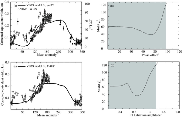
Figure 10. Similar to Figure 9, except that there the VIMS observations of corrected equivalent width (CEW; Hedman et al. 2013) are used. (a) Best-fit model to VIMS-only data is shown with solid line. Here a = 0.015 km and b = 0.25 km (Equation (3)). Black dots are ISS data replotted from Figure 9 and assuming that CEW and I/F have a simple linear relationship. (b) Misfit as a function of phase lag. (c) As for panel (a), but the best-fit line shows the libration model fitted to VIMS-only with a = 0.045 km and b = 0.228 km. (d) Misfit as a function of libration amplitude.
Download figure:
Standard image High-resolution imageFigure 10(a) also overlies the ISS data on the VIMS data, assuming the two data sets are linearly related. The two data sets show very similar behavior, but the fits to the ISS data are more constraining because they do not suffer from the VIMS data gap in the range M = 210° to M = 330°. Performing a joint fit to the combined VIMS and ISS data set produces results that are very similar to the VIMS-only fits, because there are an order of magnitude more VIMS observations than ISS.
6. DISCUSSION
Based on our modeling of ISS plume observations, we identify three potential candidate models to explain the observations: (1) the activity is controlled by right-lateral strike slip motion; (2) the activity is driven by eccentricity tides with an apparent time delay of about 5 hr; (3) the activity is driven by eccentricity tides plus a 1:1 physical libration with an amplitude of about 08 (3.5 km).
The first explanation can readily be tested by detailed geological mapping of the SPT. However, it results in a relatively poor fit to the observations (Table 2), and as a result we do not favor it at this time.
The second explanation produces a better fit, and can be explained in at least two ways. First, there may be a delay between the initial triggering of an eruption and the surface expression of that eruption. A 4 hr delay from a source at 10 km depth implies a propagation velocity of ∼0.7 m s−1. This velocity is two orders of magnitude lower than the inferred velocities of jet particles (Ingersoll & Ewald 2011). Furthermore, a detailed model of an eruption following clathrate destabilization (Halevy & Stewart 2008) predicts the vast majority of the flux occurring in the first half of the orbit, which we do not observe. However, on Earth some volcanic eruptions appear to be triggered (by earthquakes) with delays of up to a few days (Manga & Brodsky 2006). Perhaps the biggest problem with the eruptive time-delay hypothesis is that although it can explain a delayed onset of activity, the end of activity should still be determined by when the cracks close. As a result, one would expect to see activity decline steeply beyond M ∼ 180°, in conflict with the observations. Although we cannot entirely rule out the eruptive time-delay explanation, we view it as less probable than some of the alternatives.
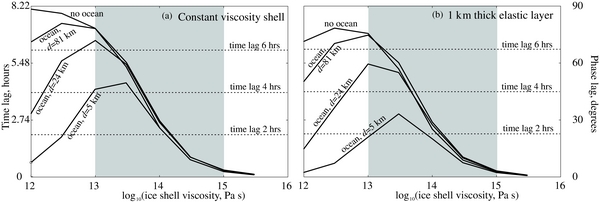
Second, the ice shell itself may display a lag in responding to the perturbing tidal potential. Viscoelastic materials experience large lags when the characteristic response time (the Maxwell time) is comparable to the forcing period (Moore & Schubert 2000). For Enceladus, this criterion yields a viscosity of ∼3 × 10¹⁴ Pa s, which is within the estimated range of convective ice shell viscosities (Goldsby & Kohlstedt 2001). Figure 11(a) plots the time lag as a function of ice shell viscosity for different ice shell thicknesses d. As expected, at ice shell viscosities <3 × 10¹⁴ Pa s, the lags can become large. Figure 11(b) presents a similar calculation, but here the top 1 km of the shell is taken to be elastic, as suggested by flexural and crater relaxation studies (Giese et al. 2008; Bland et al. 2012). Figure 11 makes it clear that a time lag of 5.1 ± 0.8 hr is compatible with a wide range of models, including those with and without oceans, as long as the ice shell is convecting.
Figure 11. Phase lag as a function of ice shell viscosity and shell thickness d. (a) Enceladus' interior structure parameters are identical to those used in Figure 3 of Nimmo et al. (2007). The shaded region gives the likely viscosity of a convecting ice shell. The phase lag was calculated from tan−1 (h2i/h2r) where h2i and h2r are the real and imaginary degree-2 Love numbers. Note that the amplitude of the tidal response (Figure 3 of Nimmo et al. 2007) is more strongly affected by the shell thickness than is the phase. The horizontal dashed lines indicate time lags for comparison with our inferred lag of 5.1 ± 0.8 hr. Calculations were performed using the method of Moore & Schubert (2000). (b) As for panel (a), but including a rigid elastic surface layer of thickness 1 km. For a synchronous satellite, the time lag and phase lag are simply related by ψ = n Δt where n is the mean motion.
Download figure:
Standard image High-resolution image
This result is based on the assumption of a spherically symmetric body. Because heating on Enceladus is apparently confined to the SPT region, and there are probably large lateral variations in shell thickness (Collins & Goodman 2007; Iess et al. 2014), this assumption may not be correct. Both the tidal stresses and the tidal heating may be affected by lateral variations in shell properties (e.g., A et al. 2014). Models taking such lateral variations into account (e.g., Behounkova et al. 2012) are certainly desirable, but are beyond the scope of the work presented here.
If the inferred shell phase lag of ∼60° is real, it implies a tidal dissipation factor, Q, of the order of unity. Q ∼ 1 is compatible with likely Enceladus interior structures (Figure 11) and implies that present-day tidal heating is occurring in the shell (though probably not at the fractures themselves). To generate the entire observed power output (Spencer et al. 2006; Howett et al. 2011) with present-day heating would require a k2 Love number ∼0.01, consistent with a thick ice shell overlying a global ocean (Nimmo et al. 2007) or a regional sea (Behounkova et al. 2012). In reality, part of this observed power likely comes from the release of stored heat (Porco et al. 2013; Matson et al. 2012), with the balance between stored heat release and tidal heat generation likely changing over time as Enceladus' orbit evolves (Ojakangas & Stevenson 1986).
While Figure 11 makes it clear that Q ∼ 1 is theoretically plausible, no other planetary body has a Q this low (the Earth's effective Q of about 12—due mainly to dissipation in the oceans—is the next lowest). Given our poor understanding of eruptive time lags (see above), it is premature to place too much credence in the low-Q hypothesis. Furthermore, if viscous relaxation on diurnal timescales is important (as a Q ∼ 1 would imply), then the elastic approach outlined in Section 3 is too simple and a full viscoelastic treatment would be required (e.g., Wahr et al. 2009; Jara-Orue & Vermeersen 2011). However, there are potential tests available. Perhaps the most straightforward is to look for regional background heat production at the south pole (in addition to the local heat sources at the tiger stripes). Detection of such regional emission would be strong evidence for present-day viscoelastic heating. A second test is to measure the small, time-dependent tidal gravity response of Enceladus, as has been done at Titan (Iess et al. 2012). Another is to look for rotation-rate variations, since a small Q implies large tidal torques.
At the moment, the simplest explanation of the observations appears to be a large 1:1 physical libration. The required amplitude is an order of magnitude larger than theoretical predictions (Rambaux et al. 2010), but those theoretical predictions assume a solid Enceladus. An Enceladus with a decoupled shell overlying a global ocean would certainly experience larger shell librations, though the rigidity of the shell would also matter (cf. Jara-Orue & Vermeersen 2014). Fortunately, the amplitude of the librations implied by our study is sufficiently large (08 = 3.5 km) that they should be readily detectable with ISS images, although so far only librations with amplitudes greater than 15 have been ruled out (Porco et al. 2006). Gravity data (Iess et al. 2014) are consistent with either a global ocean or a regional subsurface sea; detecting librations would confirm the existence of the former.
This first attempt at modeling the time variability of activity on Enceladus is undoubtedly over-simplified, and clearly does not capture all the observed behavior. In particular, there are hints of long-period changes in activity, and there are also individual spikes in the data. Both the ISS and VIMS observations show that our models do not match the spikes at M ∼ 210° (ISS rev 119) and M ∼ 30° (ISS revs 098, 121, and 127). One possible explanation is that limited tiger stripe segments are anomalously active. In particular, the M ∼ 30° spike could be explained by the tips of the Cairo and/or Damascus fractures (see Figure 8). Another possibility is that some spikes (e.g., revs 119 and 098) are due to statistical fluctuations in plume ejecta production. Such fluctuations might explain the increase in ultraviolet emissions seen from Saturn's oxygen torus (which is sourced by the Enceladus water plume) observed by the Cassini UVIS instrument (Melin et al. 2009).
For simplicity we have discussed three possible explanations for the observed plume behavior separately, but in reality some combination of processes may be operating. For instance, in theory, 1:1 physical librations of some magnitude should always accompany eccentricity tides. We defer consideration of these more complicated situations to future work.
Aside from the issue of which model (or models) best describes the variability in plume brightness, two results presented here are relevant to specific details of the eruption mechanism. First is the fact that we never see the plume entirely go away, which suggests that the source vents never completely close when the tensile stresses fall to zero and below, as the basic tidal stress model would suggest they should. The best explanation here may be the simplest: rough fracture-wall topography and boulders within the near-surface region of the fracture may prevent complete closure. That is, on average, vents narrow with increasing compressive stresses but never fully close.
The inference that the opening and closing of fractures brings about the variability in mass flux of fine particles seen by both ISS and VIMS makes it surprising that the scale height of the plume does not show systematic variations. One naively might expect that the narrowing of vents would increase the flow speed, which in turn would yield larger scale heights (provided the particle size distribution did not change). A likely solution is that the supersonic nature of the jets (e.g., Schmidt et al. 2008) needs to be taken into account. Supersonic flows have several counterintuitive properties, among them the fact that while the mass flux depends on the vent area at the so-called choke point, the velocity across this point does not (e.g., Housley 1978; Kieffer 1989). A roughly constant exit velocity, regardless of stress magnitude, appears to be required to explain the absence of systematic variations in scale height. In this case, the random scatter in our scale height data may indicate large, stochastic changes in the mass production rates of individual jets, suggested by some of our plume brightness observations (e.g., revs 119 and 098). Alternatively, the large random scatter could in principle mask any smaller underlying systematic effect due to variation in vent widths. In either case, these results will provide constraints on future models for the hydrodynamics of geyser eruptions on the SPT of Enceladus.
7. SUMMARY AND FUTURE WORK
The ISS and VIMS observations both show that jet activity varies over the tidal cycle. Our initial modeling effort suggests three possible explanations for the observations: eruptions controlled by right-lateral strike slip faulting, control by eccentricity tides plus a time delay, and control by eccentricity tides plus a 1:1 physical libration. While we cannot rule out any of these explanations, we point out that the last one does make predictions that are testable: a longitudinal libration with an amplitude of about 3.5 km should be readily detectable with ISS images. Furthermore, such a libration would necessarily imply a global subsurface ocean.
Several theoretical aspects of our approach could also be improved on in the future. Perhaps most notably, the long-period libration model which was originally developed to model rigidly responding bodies may not be appropriate for more deformable (but not fluid) bodies such as Enceladus. Likewise, it will undoubtedly be important to repeat our stress calculations using a full viscoelastic approach (cf. Wahr et al. 2009; Jara-Orue & Vermeersen 2011) and taking possible lateral variations in viscosity structure into account (cf. Behounkova et al. 2012; A et al. 2014). Of course, modeling of the eruptive behavior of Enceladus jets is in its infancy. While we find that the clathrate-destabilization model of Halevy & Stewart (2008) does not provide a good match to the observations, more work could certainly be done in this area. In particular, modeling the response of supersonic jets to changes in vent area (cf. Mitchell 2005; Ogden et al. 2008) would seem to be a fruitful avenue to explore.
Regardless of Enceladus' orbital position, the brightness of the observed plume, and the predicted normal stresses along the tiger stripe fractures, the scale height of the plume does not vary systematically in any way, although there is a lot of scatter in the results (Figure 7). These results should provide reasonable constraints on future hydrodynamical modeling of the flow responsible for producing the forest of geysers erupting from the moon's SPT.
We thank the CICLOPS staff for their assistance in planning and executing the image sequences used in this work. We thank Matt Tiscareno for software assistance in the efficient use of the JPL kernels, and Matt Hedman for fruitful conversations about the interpretation of VIMS plume data. We thank Benoit Noyelles for patient explanations of long-period librations and Emily Brodsky and Darcy Ogden for discussions of supersonic jets. We thank the reviewer, Dave Stevenson, for helpful comments. C.C.P. acknowledges support from NASA CDAP and the Cassini project, and F.N. from the CDAP-PS program.
Footnotes
- 3
We use the word "plume" to refer to the extended feature seen from a distance in ISS images, as opposed to the individual jets or geysers that are seen at very high resolution and reported on in Paper 1.