


ABSTRACT
Compositional zoning in chondrule phenocrysts records the crystallization environments in the early solar nebula. We modeled the growth of olivine phenocrysts from a silicate melt and proposed a new fractional crystallization model that provides a relation between the zoning profile and the cooling rate. In our model, we took elemental partitioning at a growing solid–liquid interface and time-dependent solute diffusion in the liquid into consideration. We assumed a local equilibrium condition, namely, that the compositions at the interface are equal to the equilibrium ones at a given temperature. We carried out numerical simulations of the fractional crystallization in one-dimensional planar geometry. The simulations revealed that under a constant cooling rate the growth velocity increases exponentially with time and a linear zoning profile forms in the solid as a result. We derived analytic formulae of the zoning profile, which reproduced the numerical results for wide ranges of crystallization conditions. The formulae provide a useful tool to estimate the cooling rate from the compositional zoning. Applying the formulae to low-FeO relict olivine grains in type II porphyritic chondrules observed by Wasson & Rubin, we estimate the cooling rate to be ∼200–2000 K s−1, which is greater than that expected from furnace-based experiments by orders of magnitude. Appropriate solar nebula environments for such rapid cooling conditions are discussed.
Export citation and abstract BibTeX RIS
1. INTRODUCTION
Most chondritic meteorites contain millimeter-sized spherical crystalline grains consisting mainly of silicate material. They are called chondrules, which are considered to have crystallized from silicate melt droplets 4.6 billion years ago in the solar nebula (Amelin et al. 2002; Kurahashi et al. 2008; Connelly et al. 2012). Since chondrules occupy about 80 vol.% of chondritic meteorites in abundant cases (Jones et al. 2000), they must have a wealth of information about the early history of our solar system. Chondrules exhibit various textural types (Gooding & Keil 1981; Weisberg 1987) and zonal structures (Nagahara 1981; Miyamoto et al. 1986; Jones & Scott 1989; Jones 1990) reflecting their different solidification conditions. Experiments simulating chondrule-melt crystallization succeeded in reproducing some textural features of chondrules, and provided information on the thermal histories that they have experienced during solidification (Nelson et al. 1972; Tsuchiyama et al. 1980; Lofgren & Russell 1986; Jones & Lofgren 1993; Tsuchiyama et al. 2004; Nagashima et al. 2006; Srivastava et al. 2010). However, the solidification processes yielding the chondrule textures remain unclear to date.
The key process of the chondrule-melt crystallization is elemental partitioning between growing phenocrysts and the remaining liquid. One of the major phenocrysts is olivine, which is composed of two crystalline end members, forsterite (Mg2SiO4) and fayalite (Fe2SiO4), and forms a complete series of solid solutions (Bowen & Schairer 1935). The solid phase is more depleted in fayalite than the co-existing liquid, implying that the liquid becomes rich in fayalite along with the growth of phenocrysts. In a similar manner, other incompatible elements such as Ca and Al are also concentrated in the liquid. The change in the liquid composition is recorded as compositional zoning in olivines. Jones (1990) showed that the zoning profile of CaO in type II porphyritic olivine chondrules in Semarkona (LL3.0) agrees with that expected by Rayleigh distillation for fractional crystallization in a closed system. The Rayleigh fractionation model allows the change in the liquid composition during solidification; however, it does not allow the compositional gradient in the liquid (see Figure 1(a)). The use of this model is justified if the crystal growth is so slow that the elements have enough time for diffusive or convective homogenization in the liquid. The timescale for the homogenization by diffusion is estimated to be τ ∼ d2/DL ∼ 103–104 s, where d ∼ 1 mm is the typical diameter of chondrules and DL ∼ 10−6–10−5 cm2 s−1 is the typical diffusivity of the liquid at the liquidus temperature of chondrules (Brady 1995). The canonical constraint on the cooling rate of porphyritic olivine chondrules, Rc ∼ 2–100 K hr−1 (Jones & Lofgren 1993), allows us to apply the Rayleigh fractionation model.
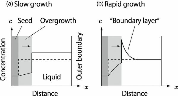
Figure 1. Transient concentration profile of iron or incompatible elements during olivine growth. (a) The case when the olivine growth is much slower than the diffusive and/or convective solute transportation in liquid. The dashed line shows an initial profile at which a seed olivine crystal is in equilibrium with the liquid. As the olivine grows, the concentration in the liquid is increased gradually but uniformly, as shown by the solid line. (b) The case when the olivine growth is much faster than the element transportation in the liquid. The elements are concentrated ahead of the moving interface and form a diffusive boundary layer.
Download figure:
Standard image High-resolution imageOn the other hand, there are lines of evidence suggesting much more rapid chondrule-melt crystallization. Yurimoto & Wasson (2002) reported that some Fe–Mg exchange but negligible oxygen–isotopic exchange occurred between a magnesian olivine phenocryst and the remainder of the chondrule. They suggested an extremely rapid cooling, say ∼105–106 K hr−1, to account for their observations according to their diffusional model. Wasson & Rubin (2003) observed low-FeO relict olivine grains in type II porphyritic chondrules and found that the grains exhibit narrow overgrowth of ∼4–10 μm in thickness accompanied with a linear compositional zoning. They discussed that the narrow overgrowth indicates much more rapid cooling than the canonical constraints. Solidification under such rapid cooling causes a compositional gradient in the liquid (see Figure 1(b)). The compositional gradient leads to significant modifications in the solidification processes such as kinetic disequilibrium in the elemental partitioning between phenocrysts and the remaining liquid (Albarede & Bottinga 1972), excessive uptake of incompatible elements in fluid inclusions (Baker 2008), isotopic fractionation (Watson & Müller 2009), and dendrite formation due to morphological instability (Mullins & Sekerka 1964). The morphological instability is considered to be the origin of barred-olivine textures in chondrules (Tsuchiyama et al. 2004).
To decipher the records of the solar system history preserved in the chondrule textures, we should obtain comprehensive understanding of the dynamics of solidification. In this paper, we concentrate on the linear zoning profile observed in overgrown olivines in chondrules (Wasson & Rubin 2003) because it suggests much more rapid cooling in their formation environment than that supposed so far. We found that the linear zoning is formed as a result of rapid solidification and that the cooling rate to reproduce the zonal slope is much greater than the canonical constraints. In Section 2, we devise a numerical model of crystal growth, which takes account of the elemental partitioning at a moving solid–liquid interface and the incomplete solute diffusion in the liquid in one-dimensional planar geometry. In Section 3, we reproduce the linear zoning profile by numerical calculations for various cooling rates. In Section 4, we derive an analytic expression that reproduces the numerical results. In Section 5, we estimate the cooling rate of chondrules and discuss solar nebula environments appropriate for chondrule formation. Conclusions are given in Section 6.
2. MODEL
2.1. Thermodynamics of Olivine
We simulate the olivine growth in a manner consistent with a thermodynamical model of olivine. We consider a simple binary system for olivine composed of two crystalline end members, forsterite (Mg2SiO4) and fayalite (Fe2SiO4). Although natural ferromagnesian olivines contain minor amounts of additional divalent cations including Ca, Mn, Ni, and Co (Hirschmann 1991), we ignore these minor elements as a first step. The fayalite contents in solid and liquid in equilibrium are given by an ideal solution model in good approximation (Bowen & Schairer 1935). The concentration c is defined by an atomic ratio Fe/(Mg + Fe). The equilibrium concentrations in liquid and solid,  and
and  , at temperature T are given by
where
Here, subscripts A and B stand for pure forsterite (Mg2SiO4) and pure fayalite (Fe2SiO4), respectively; LA, B, their molar latent heats of crystallization; TA, B, their absolute melting points; and R, the gas constant. The parameters are set as LA = LB = 58.6 kJ mol−1 (Bowen & Schairer 1935), TA = 2163 K, and TB = 1490 K. The phase diagram is shown in Figure 2. Values of the equilibrium concentrations  and
and  are listed in Table 1. Note that the equilibrium partitioning coefficient,
  , is less than unity for all T.
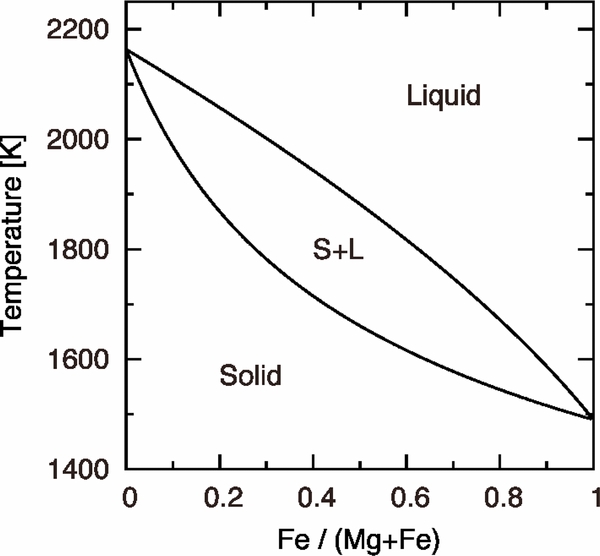
Figure 2. Phase diagram of the Mg2SiO4–Fe2SiO4 system.
Download figure:
Standard image High-resolution imageTable 1. Parameter Values Deduced from the Phase Diagram for Various Temperatures T
| T |  |
 |
k0 | ΔTc |
|---|---|---|---|---|
| (K) | (K) | |||
| 1500 | 0.990 | 0.960 | 0.969 | 7.6 |
| 1600 | 0.886 | 0.640 | 0.722 | 80 |
| 1700 | 0.764 | 0.426 | 0.557 | 144 |
| 1800 | 0.625 | 0.277 | 0.443 | 194 |
| 1900 | 0.471 | 0.170 | 0.360 | 224 |
| 2000 | 0.303 | 0.091 | 0.299 | 220 |
| 2100 | 0.121 | 0.031 | 0.253 | 142 |
Notes. Here,  and
and  are equilibrium concentrations in liquid and solid, respectively;
  , equilibrium partitioning coefficient; ΔTc, temperature difference between liquidus and solidus for given concentrations
  .
.
Download table as: ASCIITypeset image
2.2. Basic Equations
Crystal growth associated with solute diffusion in a liquid has been formulated as a moving boundary problem to describe the compositional zoning (Tiller et al. 1953; Smith et al. 1955). Let us consider a crystal growing toward x direction. We also take another coordinate x' comoving with the solid–liquid interface; the origin x' = 0 is fixed at the interface. We neglect the solute diffusion in solid (x' < 0) because the diffusivity in the solid is much smaller than that in the liquid (Dohmen et al. 2007). The diffusion equation for the concentration cL(x'; t) in the liquid is given by
where V(t) is the time-dependent growth velocity and DL is the diffusivity in the liquid. We neglect convective solute transportation in the liquid in Equation (3). A coordinate fixed with the solid, x, is then
where d(t) is the position of the interface on the coordinate x.
Equation (3) must be solved subject to the initial condition given by

the boundary conditions given by

at x = ∞, and
at x' = 0 for any t (Lasaga 1982), where cL0 is the initial concentration in the liquid and cLi and cSi are the concentrations at the interface on the liquid and solid sides, respectively. Tiller et al. (1953) and Smith et al. (1955) set cSi = k0cLi in Equation (7), where k0 is a constant partitioning coefficient. However, k0 depends on the temperature T in general and varies with T in the course of cooling. Furthermore, they set V to be constant. But V actually varies with T and this determines the zoning profile we are interested in. Thus, we must determine the time variation of V as well as the concentration cL. In the narrow regions on both sides of the solid–liquid interface, we can expect equilibrium partitioning to be realized. Hence, we assume local equilibrium partitioning, namely,

With the use of Equation (8), the boundary condition (7) is written as
2.3. Numerical Procedure
We consider the spatial domain  for the numerical simulation, where
  is set to be so large that
  is not affected by the diffusive boundary layer. The domain is divided into N grid cells of uniform width,
  . The time direction is also discretized by a constant interval Δt.
  denotes the concentration at the grid cell i at the time step n. From Equation (3), we obtain the difference equation:
where η = DLΔt/Δx'2 and v = VΔt/Δx'. The term  denotes the boundary condition given by Equation (9). For i = N, we use
  . We use the first-order upwind differential scheme for the advection term under the assumption of v > 0. Note that v is not given a priori in our model but is determined to satisfy a local equilibrium condition at x' = 0:

We need an iterative scheme to obtain v as described below.  denotes a trial value of v at kth iterative step. We obtain the trial solution of concentration
  by
by
If  satisfies the condition given by Equation (11), we can proceed to the next time step with
  . If
. If  , which suggests that large
  causes over-partitioning, we should choose
  smaller than
  . In contrast, if
  , we should choose
  larger than
  . We use
for the next trial. The condition for convergence is taken to be

The change in the threshold value does not affect the solution significantly. In this paper, we use  , N = 104, Δx' = 10 nm, and Δt = 10−6 s.
2.4. Computational Setting
We consider a solid–liquid equilibrium at T = T0 at the beginning. The initial liquid concentration is given by  . We decrease T at a constant rate Rc and continue the numerical procedure until the zoning profile in the solid forms obviously. We carry out the numerical simulation for different sets of parameters T0 and Rc to investigate how the zoning profile depends on these parameters. For simplicity, we use a constant diffusivity of DL = 10−5 cm2 s−1, which is a typical value for silicate melt (Brady 1995).
3. RESULT
3.1. Initial Transient and Diffusion Layer
Figure 3 shows a numerical result for T0 = 1900 K and Rc = 103 K s−1. Panel (a) shows the concentrations in solid and liquid phases. The dashed, dotted, or dash–dotted curve shows a snapshot of concentration cL(x; t) in the liquid phase at every 50 K decrease in temperature. The horizontal axis indicates x, not x', so the solid–liquid interface is not fixed at the origin. As the temperature decreases, the interface moves rightward. Figure 3(a) shows that cL rises ahead of the moving interface as a result of the partitioning. The diffusive boundary layer appears when the solute diffusion is insufficient to homogenize the concentration in the liquid. The appearance of the diffusive layer plays an important role in determining growth velocity and a zoning profile in the solid.
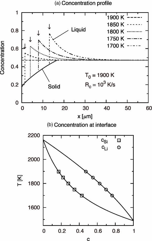
Figure 3. Numerical result of solidification of olivine under constant cooling rate for T0 = 1900 K and R0 = 103 K s−1. (a) The solid curve shows the concentration profile in the solid phase. Other curves show the snapshots of concentration in the liquid phase at every time where the temperature decreases by 50 K; note that the horizontal axis is not x' but x = x' + d(t), where d(t) is the position of the solid–liquid interface at each moment (indicated by arrows). (b) The symbols show the calculated concentrations cSi (solid phase) and cLi (liquid phase) at the interface as a function of decreasing temperature. The solid curves are the solidus and liquidus of the ideal binary system of olivine composition.
Download figure:
Standard image High-resolution imageThe solid curve shows a series of cSi formed as a result of the motion of the interface. This is the zoning profile recorded in the solid immediately after its formation; in fact, a solid phase has non-zero diffusivity, so the zoning profile will be modified thermally (Miyamoto et al. 1986). In this study, we neglect the solute diffusion in the solid. Note that cSi increases monotonically with x and exceeds the initial liquid concentration cL0 = 0.471 at x = 16.5 μm. The region in which the composition changes steeply is called an initial transient in alloy solidification (Smith et al. 1955). Here, we define the region in which cS < cL0 as the initial transient; its width is df = 16.5 μm in this case.
Figure 3(b) plots cSi and cLi on the phase diagram during solidification. Note that both cSi and cLi vary respectively along the solidus and liquidus curves with the decrease in temperature. This confirms that the local equilibrium condition is satisfied in the calculation.
3.2. Time-dependent Growth Velocity
Figure 4 shows the interface position d(t) for T0 = 1900 K and Rc = 103 K s−1 as a function of time, indicating that the crystal growth is accelerated with time. Let us assume that the growth velocity  is expressed by

where V0 is the initial growth velocity and t0 is a time constant. The physical grounds of Equation (15) will be discussed in Section 4.1. Integration of Equation (15) leads to

where we put d(0) = 0. We fit the numerical result using Equation (16) and obtain best-fit values of V0 = 26.2 μm s−1 and t0 = 0.124 s for T0 = 1900 K and Rc = 103 K s−1. Note that Equation (16) reproduces the numerical result excellently in almost the entire region of the initial transient.

Figure 4. Interface position df(t) as a function of time for T0 = 1900 K and Rc = 1000 K s−1 (open circles). The solid curve shows the best fit by Equation (16).
Download figure:
Standard image High-resolution image3.3. Dependence on Cooling Rate
We carry out calculations for a wide range of T0 and Rc. Numerical results are summarized in Table 2. Figure 5 shows dependence of the initial transient parameters of df (panel a), V0 (panel b), and t0 (panel c) on Rc. Results for different T0 values are shown by using different symbols (see the legend in panel a). We find that all these parameters show a power-law dependence on Rc, namely,  ,
,  , and
, and  . The power-law dependence is observed for a wide range of T0.
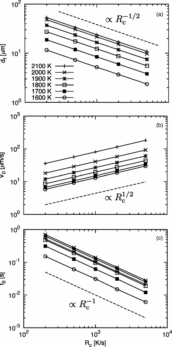
Figure 5. Dependence of the initial transient parameters—(a) width of the initial transient, df, (b) initial growth velocity V0, and (c) time constant t0—on the cooling rate Rc. The legend gives the values of the initial temperature T0.
Download figure:
Standard image High-resolution imageTable 2. Numerical Results of Moving Boundary Problem for Various Initial Temperatures T0 and Cooling Rates Rc
| T0 | Rc | tf | df | V0 | t0 |
|---|---|---|---|---|---|
| (K) | (K s−1) | (s) | (μm) | (μm s−1) | (s) |
| 2100 | 5000 | 0.028 | 10.4 | 170 | 0.020 |
| 2000 | 0.071 | 16.6 | 109 | 0.051 | |
| 1000 | 0.142 | 23.6 | 78.0 | 0.103 | |
| 500 | 0.284 | 33.5 | 55.4 | 0.206 | |
| 200 | 0.709 | 53.1 | 35.2 | 0.515 | |
| 2000 | 5000 | 0.044 | 9.42 | 87.4 | 0.028 |
| 2000 | 0.110 | 15.0 | 56.0 | 0.069 | |
| 1000 | 0.220 | 21.3 | 39.8 | 0.139 | |
| 500 | 0.441 | 30.2 | 28.3 | 0.278 | |
| 200 | 1.10 | 47.9 | 18.0 | 0.696 | |
| 1900 | 5000 | 0.045 | 7.30 | 57.5 | 0.025 |
| 2000 | 0.112 | 11.6 | 36.8 | 0.062 | |
| 1000 | 0.225 | 16.5 | 26.2 | 0.124 | |
| 500 | 0.449 | 23.4 | 18.6 | 0.249 | |
| 200 | 1.12 | 37.0 | 11.8 | 0.624 | |
| 1800 | 5000 | 0.039 | 5.38 | 41.5 | 0.019 |
| 2000 | 0.097 | 8.57 | 26.6 | 0.047 | |
| 1000 | 0.194 | 12.2 | 18.9 | 0.095 | |
| 500 | 0.388 | 17.2 | 13.4 | 0.190 | |
| 200 | 0.971 | 27.3 | 8.53 | 0.476 | |
| 1700 | 5000 | 0.029 | 3.75 | 32.0 | 0.012 |
| 2000 | 0.072 | 5.97 | 20.5 | 0.031 | |
| 1000 | 0.144 | 8.48 | 14.6 | 0.062 | |
| 500 | 0.288 | 12.0 | 10.4 | 0.124 | |
| 200 | 0.720 | 19.1 | 6.60 | 0.310 | |
| 1600 | 5000 | 0.016 | 2.29 | 27.5 | 0.0060 |
| 2000 | 0.040 | 3.65 | 17.7 | 0.015 | |
| 1000 | 0.080 | 5.19 | 12.6 | 0.030 | |
| 500 | 0.161 | 7.37 | 9.00 | 0.061 | |
| 200 | 0.402 | 11.7 | 5.73 | 0.152 |
Notes. Here, tf is the time at which the solid concentration reached the initial liquid concentration; df, the position of the solid–liquid interface at t = tf; V0, initial growth velocity; t0, the time constant.
Download table as: ASCIITypeset image
4. ANALYSIS OF COMPOSITIONAL ZONING
In the previous section, we obtained the initial transient parameters df, V0, and t0 as a function of Rc. In this section, we derive analytic expressions for these initial transient parameters on the basis of the local equilibrium condition at the moving solid–liquid interface. We shall show that the analytic expressions well reproduce the numerical results for wide ranges of T0 and Rc.
4.1. Physical Grounds of the Exponential Time Variation of the Interface Velocity
The numerical simulation yielded a remarkable result that the interface velocity increases exponentially with time for a constant rate of temperature decrease. We investigate its physics briefly in this subsection. Figure 6(a) shows the motion of the solid–liquid interface followed by the change in the concentration profile during a short duration Δt. The black and red curves are the profiles before and after the motion of the interface, respectively. The concentration excess (see Appendix A.1) in the liquid is evaluated to be
where δ is a width of the diffusive boundary layer and is approximately constant. AL increases monotonically with decreasing T because of the ejection of a portion of the solute from the solidified layer. On the other hand, the amount of solute ejected from the solidified layer during Δt is given (see Appendix A.1) by

The solute conservation requires ΔAS(t) = AL(t + Δt) − AL(t), hence, we obtain
where Rc = −dT/dt and  . Here, k0 can be regarded as a constant around T ∼ T0. Since solidus can be approximated by a straight line around T ∼ T0 (see Figure 6(b)), we obtain
where ΔTc is the temperature difference between liquidus and solidus at a given concentration. Using Equation (20), the time variation of V is evaluated to be
where  around T ∼ T0. Equation (21) indicates that V increases exponentially with t at least in the early stage of the growth, which is in harmony with Equation (15). It is also indicated that the time constant t0 is on the order of ΔTc/Rc.
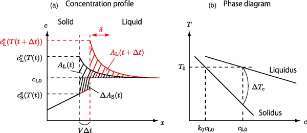
Figure 6. Schematic illustrations for explaining the physics of exponential growth velocity. (a) Change in the concentration profiles in solid and liquid during a short duration Δt. A typical width of the diffusive boundary layer in the liquid is expressed by δ. (b) The phase diagram magnified at T ∼ T0.
Download figure:
Standard image High-resolution image4.2. Time Constant
We showed t0 ∼ ΔTc/Rc ≡ tsol, where tsol is called a solidification time, that is, a period required for the temperature to decrease from the liquidus to the solidus for a given cL0. In Figure 7(a), we compare tsol with t0 calculated for all input parameters. Each symbol corresponds to a result for a set of T0 and Rc. It is found that all symbols are aligned on a straight line with a slope of unity, suggesting that t0 is proportional to tsol for wide range of T0 and Rc. The symbols align along the t0 = tsol/2 line. Hence, including the numerical factor, t0 is expressed by
Note that t0 is inversely proportional to Rc.
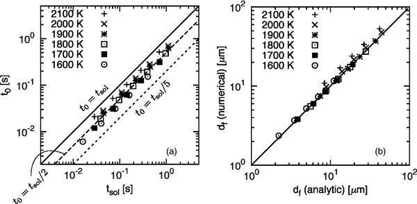
Figure 7. Comparison between the analytic formulae and the numerical results. (a) The time constant t0 and the solidification time tsol. The solid, dashed, and dotted lines correspond to t0 = tsol, t0 = tsol/2, and t0 = tsol/5, respectively. (b) Comparison of the width df of the initial transient calculated by Equation (24) (analytic) with df obtained by the numerical simulation (numerical).
Download figure:
Standard image High-resolution image4.3. Width of the Initial Transient
Taking the exponential acceleration of the growth velocity into account, the solute distribution in the crystal in the initial transient is expressed (see the Appendix) by
where we used Equation (22). Equation (23) shows that the solute concentration increases linearly with distance x in contrast to the Rayleigh fractionation (Rayleigh 1896) and Smith's model (Smith et al. 1955). From cS(df) = cL0, we immediately obtain the width of the initial transient expressed by
Note that df is proportional to  in agreement with the numerical results shown in Figure 5(a). Figure 7(b) shows that Equation (24) well reproduces the numerical results.
5. DISCUSSION
5.1. An Example of the Estimation of the Cooling Rate
As an example of the application of the present theory, we estimate a cooling rate by analyzing a zoning profile recorded in chondrules. Wasson & Rubin (2003) observed zoning profiles of olivines in type II chondrules in Y-81020 carbonaceous chondrite. They found that some large (>40 μm) olivine phenocrysts have low-FeO relicts near the centers and surrounding FeO-rich margins. In the margin, the fayalite composition linearly increases from c ≃ 0.22–0.39 to ≃ 0.38–0.77 within the thickness of ≃ 2–12 μm. In other words, the compositional gradient is ∼102–103 cm−1. Wasson (2004) assumed that the narrow FeO-rich margins were produced by diffusion-controlled overgrowth of the phenocrysts during the final melting event and estimated the cooling rate to be ∼103 K s−1. However, his estimation includes an uncertain parameter of "blocking" temperature at which the overgrowth stops; it must depend on the cooling rate. Furthermore, he did not explain the origin of the linear zoning profile.
Our model naturally explains the linear zoning profile (see Figure 3(a)) and can estimate the cooling rate without introducing an uncertain parameter. From Equation (23), we obtain
where dcS/dx is the compositional gradient in the linear zoning profile. From this, the cooling rate is estimated to be Rc ≈ 200–2000 K s−1 for DL = 10−6–10−5 cm2 s−1, ΔTc = 200 K, k0 = 0.4, cL0 = 0.5, and dcS/dx = 300 cm−1. The Rc value is on the same order of magnitude as that estimated by Wasson (2004) incidentally, although our theory clearly identifies the origin of the linear zoning profile. These estimates are higher by orders of magnitude than the cooling rates of 0.01–1 K s−1 inferred from furnace-faced experiments (Jones et al. 2000; Hewins et al. 2005).
5.2. Implications for Chondrule-forming Environments
Aerodynamic drag heating induced by nebula shocks is one of the plausible mechanisms to melt chondrule precursor silicate grains (Wood 1984). This mechanism accounts for various properties of chondrules such as appropriate cooling rates inferred by furnace-based experiments (Hood & Horanyi 1991; Hood & Ciesla 2001; Desch & Connolly 2002; Miura & Nakamoto 2006; Morris et al. 2009; Morris & Desch 2010; Morris et al. 2012), maximum temperature up to the melting point (Iida et al. 2001), size distribution (Susa & Nakamoto 2002; Miura & Nakamoto 2005; Kato et al. 2006; Miura & Nakamoto 2007), oblate-shaped chondrules (Miura et al. 2008a), and formation of compound chondrules (Ciesla 2006; Miura et al. 2008b; Yasuda et al. 2009).
The aerodynamic heating requires the chondrule-forming region to be optically thick for the dust thermal radiation to satisfy the cooling rate constraint inferred by the furnace-based experiments (≲ 103 K hr−1); inefficient radiative losses in the dusty cloud result in a much slower cooling rate than that expected from the radiative cooling in vacuum (Hood & Ciesla 2001; Desch & Connolly 2002). However, our new constraint given by Equation (25) suggests an extremely rapid cooling as fast as that expected from the free radiation. The extremely rapid cooling supports shock waves produced in the optically thin environment: planetesimal bow shocks (Hood 1998; Ciesla et al. 2004; Hood et al. 2005), nebula shocks in less-dusty environments (Iida et al. 2001), and shock waves induced by X-ray flares (Nakamoto et al. 2005). It has been believed that most of chondrules were melted multiple times in the early solar nebula (Jones et al. 2000) and the FeO-rich overgrowth on the relict porphyritic olivines records the final melting event in the multiple heating episodes (Wasson & Rubin 2003). The extremely rapid cooling on chondrules at the final melting event is consistent with the fact that the solar nebula gradually became optically thin due to accumulation of dust particles onto the forming planets.
Lightning discharges are one of the leading candidates satisfying the extremely rapid cooling constraint. Most models of the nebular lightning focused on the mechanism of charge separation and initiation of electrical breakdown (Gibbard & Levy 1997; Pilipp et al. 1998; Desch & Cuzzi 2000). On the other hand, Horányi et al. (1995) examined the thermal history of chondrule precursor dust particles in the optically thin expanding discharge channel quantitatively. According to Horányi's model, the precursor particle heated above its melting point solidifies within about 1 s, which corresponds to a cooling rate of a few 100 K s−1 and meets the constraint given by Equation (25).
6. CONCLUSION
We simulated numerically rapid growth of an olivine phenocryst from a silicate melt in consideration of the transient compositional gradient in the liquid. This simulation is a mimicry of the overgrowth of relict olivine in a chondrule melt droplet at the last of the multiple heating episodes. The numerical results showed that the linear Mg–Fe zoning forms in the overgrown region. We found that the compositional gradient in the linear zoning is proportional to the square root of the cooling rate. We derived analytic formulae that reproduce the numerical results for wide ranges of solidification conditions. Applying the formulae to the linear Mg–Fe zoning observed in low-FeO relict olivine grains in type II porphyritic chondrules (Wasson & Rubin 2003), we showed that the last heating event experienced by this chondrule is much more rapid than that expected from the traditional furnace-based experiments by orders of magnitudes.
The most important outcome of this paper is that we proposed a new method for estimating the cooling rate from zoning profiles preserved in chondrules, namely, the analytic relations between the compositional zoning profile and the growth conditions of crystals. Although we limited ourselves in this paper to a binary system of olivine composition for clarity, the relations enable one to reveal the growth conditions, in particular, the cooling rate at the formation of chondrules. The cooling rate is one of the most important but undetermined key parameters in astromineralogy and in clarifying thermal history in the solar nebula. The theory can easily be straightforwardly extended for ternary or general multicomponent systems. Our approach may provide a new diagnostic method for compositional zonings in rapidly grown minerals.
This work was partially supported by Tohoku University Global COE Program "Global Education and Research Center for Earth and Planetary Dynamics." H.M. was supported by JSPS KAKENHI Grant Number 23740330 and T.Y. by the Grant-in-Aid Scientific Research on Innovative Areas (23103004) from MEXT.
APPENDIX: ANALYTIC MODEL OF LINEAR ZONING
We derive an analytic expression of the compositional zoning profile in the initial transient for binary systems when the growth velocity increases exponentially with time after the onset of solidification.
A.1. Outline of the Model
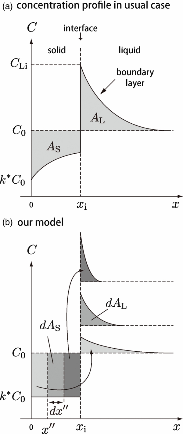
Consider a system composed of solid and liquid phases in equilibrium. Figure 8(a) shows solute concentration distributions in solid and liquid phases during solidification. Initially, the region of x < 0 was occupied by the solid phase and x > 0 by the liquid phase. The liquid was homogeneous with a constant concentration cL0. As the solidification proceeds, the interface moves rightward and a portion of the solute is ejected from the solidified region and added to the adjacent liquid region. The solute added to the liquid is transported away from the interface afterward by diffusion. When the interface reaches x = xi, the total amount of solute AS ejected from the solidified region is given by
This must be equal to that added to the liquid given by
from the conservation of solute content. Smith et al. (1955) derived analytic solutions of cS(x) and cL(x) assuming that the interface moves at a constant speed.
Figure 8. Schematic of the model used to derive the solute concentration profile. (a) The concentration distributions in the solid and liquid in a general case. (b) Our model. At any instant, the solute concentration profile in the liquid phase is considered to be given by the superposition of the concentrations of solute elements transferred from the solid phase. The solute element transferred earlier will diffuse farther from the interface (light gray region).
Download figure:
Standard image High-resolution image
We derive a solution cS(x) in the initial transient for the case that the velocity changes with time. Let us consider an infinitesimal solute element dAS ejected from the solidified region during the movement of the interface from x = x'' to x = x'' + dx'' (see Figure 8(b)). The solute element dAS transferred to the liquid diffuses toward x > xi and has a distribution dcL(x) in the liquid as a result. From the mass conservation, dAS must be equal to
The distribution dcL(x) has a typical diffusion length xD given by  , where t'' is the time elapsed after the ejection; the solute element ejected earlier has longer t''. By determining dAS, dAL, dcL(x), xD, and t'' properly, we obtain an expression for cS(x).
A.2. Derivation
We assume that dcL is given by

where B is a constant and x' = x − xi is the distance measured from the interface to the point concerned in the liquid. B is determined from the mass conservation dAS = dAL. From Equation (A4), we obtain
On the other hand, dAS is given by
where we neglect the spatial variation in cS and set cS(x) = k0cL0. This assumption is valid in the early phase of the initial transient because the variation in cS is much smaller than cL0 − cS(x). By equating Equations (A5) and (A6), we obtain
The position of the interface is given by  since
since  . Therefore, the period for the interface to move from x = x'' to x = xi is given by
Therefore, the concentration in the liquid at the interface is calculated to be
with the use of Equations (A4), (A7), (A8), and
Here,  is the error function. Finally, we obtain the concentration profile cS = k0cLi in the solid in the early phase of the initial transient by
For xi ≫ V0t0, cS is approximated by
Although Equation (A12) gives slightly smaller values of cS than that given by Equation (A11), the difference is less than ∼25% for any xi for the range of the parameter values listed in Table 2. Equation (A12) is accurate enough for an order of magnitude estimation.