


ABSTRACT
We present a study of the HH 110/270 system based on three sets of optical images obtained with the ESO New Technology Telescope, the Subaru Telescope, and the Hubble Space Telescope (HST). The ground-based observations are made in the Hα and [S ii] emission lines and the HST observations are made in the Hα line only. Ground-based observations reveal the existence of nine knots, which have not been previously discussed and offer some important insight into the HH 110/270 history. We perform a kinematic study of the HH 110/270 system and an analysis of its emission properties. We measure proper motions of all the knots in the system. Four of the newly identified knots belong to the HH 270 jet. Their positions indicate that the jet's axis changed its direction in the past. We speculate that similar changes may have occurred many times in the past and this could be part of the reason for the unusual structure of the HH 110 jet. The HST observations allow us to resolve individual knots into their substructures and to measure their proper motions. These measurements show that the knots are highly turbulent structures. Finally, we report the discovery of four new Herbig-Haro (HH) objects located near the HH 110/270 system.
Export citation and abstract BibTeX RIS
1. INTRODUCTION
The molecular cloud L 1617 forms a part of the large Orion B complex that spans ∼10° over the sky. Several Herbig-Haro (HH) jets are found originating from the L 1617 cloud. The HH 110 jet is probably the most enigmatic of them all. It was discovered by Reipurth & Olberg (1991), who described it as a 3' long sinuous jet extending roughly in the north–south direction (position angle (P.A.) ∼ 194°). This corresponds to about 0.45 pc at the then assumed distance of 460 pc. In this paper, we use the slightly smaller distance of 400 pc. The jet is composed of numerous knots that are embedded in a faint diffuse emission, which outlines the whole flow. The HH 110 jet starts as a narrow, well collimated flow but it gradually widens and develops a wiggling structure. The observations of Reipurth & Olberg (1991) at IR and millimeter wavelengths failed to reveal any obvious driving source of the HH 110 jet.
Reipurth et al. (1996) reported the discovery of the nearby HH 270 jet, northeast of HH 110. Five HH 270 knots were discovered. The IRAS 05489+0256 Class I source was suggested as the flow's driving source. The authors measured proper motions of the HH 110 jet and of the HH 270A knot. Based on the mutual orientation of the axes of both flows and the proper motion measurements, it was proposed that HH 270 and HH 110 jets share a common energy source. In order for this to be possible, the authors suggested that the HH 270 jet suffers a grazing collision with a nearby molecular cloud and then reappears as the HH 110 flow.
Several studies of the HH 110/270 system at millimeter and centimeter wavelengths were performed later (e.g., Olberg 1997; Rodríguez et al. 1998; Sepúlveda et al. 2011). No object that could be the driving source of the HH 110 jet was found near its apex. It was shown that HH 110 is located at the southeastern edge of a molecular core and that its origin coincides with the point of presumed deflection of the HH 270 flow. Also, another molecular core was found with its peak coinciding with the position of the HH 270/VLA 1 source.
Spectroscopic observations of the HH 110 jet have been performed by Riera et al. (2003a, 2003b) and López et al. (2005, 2010). It was found that the radial velocities in HH 110 in general become more blueshifted and total velocities diminish further away from the HH 110A knot. The estimated angle between the jet's axis and the plane of the sky varies between 9° and 25°. The whole HH 110 jet exhibits a complex spatial distribution of physical conditions. These studies support the idea of the HH 110 jet being a pulsed, deflected jet that is propagating in an inhomogeneous ambient medium.
Analytic and numerical models have been made in order to explain the structure of the HH 110 jet (e.g., Cantó & Raga 1991; Cantó et al. 2003; Raga & Cantó 1995, 1996; Raga et al. 2002). It was found that a grazing collision of a jet with a dense molecular cloud core would produce a deflected jet. At the same time, the colliding jet would start to drill a cavity into the core, eventually causing the deflected jet to disappear. Hence, in this model the deflected jet is a temporary phenomenon that occurs at the beginning of the jet–cloud collision. Its duration can be prolonged if the colliding jet has a time-dependent ejection axis (e.g., a precession). In the case of a jet with varying ejection velocity, the working surfaces survive the collision and can be seen as coherent entities at larger distances from the point of impact.
The nature of the HH 110/270 system was also studied with laboratory experiments (Coker et al. 2007; Hartigan et al. 2009). Their results agree with the idea of HH 110 being a product of a pulsed jet that interacts with a molecular cloud core.
In this paper, we study the structure of the HH 110/270 system and the proper motions of the knots therein by using three sets of optical images. The first is a set of Hα and [S ii] λ6716+6731 maps obtained with the ESO New Technology Telescope (NTT) in 1991. The second set consists of two images obtained with the Subaru Telescope in 2006 in the same emission lines. The last set is two Hα image mosaics obtained with the Hubble Space Telescope (HST) in 2004 and 2005. These are the only images of HH 110 obtained with the HST and as such they are the highest-resolution images of the object. With these images we were able to perform more accurate measurements of proper motions of individual knots. The proper motions of some of the knots were determined for the first time. The high angular resolution of the HST images allowed us to estimate the level of turbulence in the HH 110 jet.
2. OBSERVATIONS
In this section, we provide a detailed description of the observations used in this paper. A summary of all of the exposures is given in Table 1.
Table 1. The Observation Log
| Date | Total | Telescope | Instrument | Central | Δλ |
|---|---|---|---|---|---|
| Exposure Time | Wavelength (Å) | (Å) | |||
| 1991 Jan 7 | 45 minutes | NTT | EMMI | 6568 | 33 |
| 1991 Jan 7 | 45 minutes | NTT | EMMI | 6728 | 75 |
| 2006 Jan 4 | 60 minutes | Subaru | Suprime-Cam | 6600 | 100 |
| 2006 Jan 5 | 60 minutes | Subaru | Suprime-Cam | 6712 | 120 |
| 2004 Jan 21 | 82 minutes | Hubble | ACS | 6580 | 75 |
| 2005 Nov 13 | 32 minutes | Hubble | ACS | 6580 | 75 |
Download table as: ASCIITypeset image
2.1. NTT Images
Two narrowband images in the Hα and [S ii] λ6731+6716 Å emission lines were obtained with the ESO NTT on 1991 January 7, using the ESO Multi Mode Instrument (EMMI), and a CCD pixel scale of 0 166 pixel−1. The central wavelengths and widths of the two filters were 6568, 6728 Å and 33, 75 Å, respectively. The total integration time of each of the images was 45 minutes. The standard basic data reduction procedures were carried out (bias subtraction and flat fielding). The average FWHM of the point-spread function of the images is 11.
2.2. Subaru Images
Observations with the Subaru Telescope were carried out on 2006 January 4 (Hα image) and on 2006 January 5 ([S ii] image) using the Subaru Prime Focus Camera (Suprime-Cam). This camera is located at the prime focus of the Subaru Telescope, and has a pixel scale of 020 pixel−1. Two narrowband filters with central wavelengths of 6600 Å and 6712 Å and FWHMs of 100 Å and 120 Å were used. Both images are 1 hr exposures. Data reduction was performed using IRAF. The standard basic data reduction procedures were carried out (i.e., bias and dark subtraction, flat fielding, and distortion correction). The images were then stacked using the IRAF MSCRED, MSCSETWCS, MSCZERO, and GREGISTER packages. The images in Figure 1 show a region around HH 110 and are subimages of larger mosaics. The FWHM of the point-spread function of the images is 11 for the Hα image and 066 for the [S ii] image.

Figure 1. Images obtained on 2006 January 4 and 5 with the Subaru Telescope using the Subaru Prime Focus Camera in Hα (top) and [S ii] λ6716+6731 (bottom) emission lines. Both images are 60 minute exposures. The angular size of the images is 6 2 × 64. North is up and the east is left.
Download figure:
Standard image High-resolution image2.3. HST Images
Observations with the HST (Figure 2) were carried out on two occasions: the first observation was made on 2004 January 21 and the second one on 2005 November 13. The time elapsed between the two images is 661 days (1.81 years). The Advanced Camera for Surveys (ACS) in the Wide Field Channel (WFC) configuration and imaging mode was used. The WFC scale is 005 pixel−1. A narrowband Hα filter F658N with central wavelength 6580 Å and FWHM ∼ 75 Å was used. While the 2005 image was obtained by combining three 32 minute exposures, the 2004 image is a single 82 minute exposure. Additional routines were used in order to remove cosmic rays in the 2004 image. The FWHM of the point-spread function of stars in both images is 014.

Figure 2. Images from the HST using the Advanced Camera for Surveys (ACS) were obtained on 2004 January 21 (top) and 2005 November 13 (bottom) with exposure times of 82 and 36 minutes, respectively. The angular size of the images is ∼9'. In both cases the Hα filter was used. North is up and the east is left.
Download figure:
Standard image High-resolution image3. METHODS AND RESULTS
3.1. Structure
In the case of HH 110, we follow the nomenclature used in the literature (see, for example, Reipurth et al. 1996; López et al. 2005) for the previously known knots. We identify five new knots (see Figure 3): knot P' lies between the already known knots P and Q and R' lies 12'' north of knot R. Knots T, U, and V lie 13'', 31'', and 64'' southwest of knot S, respectively. The knots A and V lie 222'' (37) apart in the sky, which at an assumed distance of 400 pc corresponds to 0.43 pc.
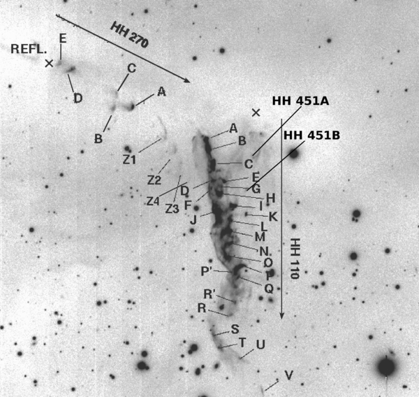
Figure 3. Knots of HH 270, HH 110, and HH 451 (Subaru Telescope image). The object marked as REFL. is a reflection nebula (see Reipurth et al. 1996) and is the counterlobe to where the HH 270 jet exits the molecular cloud. The two crosses mark the positions of the radio sources discovered by Rodríguez et al. (1998).
Download figure:
Standard image High-resolution imageKnots A–E of HH 270 were already studied before. In this work, we examine additional four knots, named Z1, Z2, Z3, and Z4. These knots were first mentioned by Reipurth et al. (1996) as a chain of knots labeled with the letter Z (see also Choi & Tang 2006). They lie 39'', 53'', 65'', and 81'' southwest of knot HH 270A. The coordinates of all newly discovered knots are given in Table 2.
Table 2. Coordinates of Newly Labeled Knots and Newly Discovered HH Objects
| Knot | R.A. | Decl. |
|---|---|---|
| (° ' '') | (° ' '') | |
| HH 110 | ||
| P' | 5 51 24 | +2 53 44 |
| R' | 5 51 24 | +2 53 18 |
| T | 5 51 25 | +2 52 40 |
| U | 5 51 24 | +2 52 31 |
| V | 5 51 23 | +2 52 03 |
| HH 270 | ||
| Z1 | 5 51 28 | +2 55 42 |
| Z2 | 5 51 27 | +2 55 28 |
| Z3 | 5 51 27 | +2 55 18 |
| Z4 | 5 51 27 | +2 55 02 |
| HH 451 | ||
| A | 5 51 23 | +2 55 25 |
| B | 5 51 23 | +2 54 55 |
| C (HH 110 K) | 5 51 23 | +2 54 35 |
| HH 490 | ||
| A | 5 51 23 | +2 47 44 |
| B | 5 51 22 | +2 48 31 |
| C | 5 51 21 | +2 48 10 |
| Others | ||
| HH 1032 | 5 51 42 | +2 45 36 |
| HH 1033 | 5 51 08 | +2 41 52 |
| HH 1034 | 5 51 04 | +2 48 26 |
| HH 1035 | 5 50 40 | +2 47 10 |
Download table as: ASCIITypeset image
The HH 270 jet appears bent around the Z1 knot. The P.A. of the axis defined by knots A–E is ∼240°, while the one defined by the knots Z1, Z2, Z3, and Z4 is ∼210°. The average P.A. of the proper motion vectors of the first group of knots is ∼240° and the corresponding P.A. for the second group is ∼249° (proper motions of the Z4 knot were not measured, since this knot does not appear in the NTT images).
3.2. [S ii] versus Hα Emission
Figure 4 was obtained by subtracting the Subaru [S ii] image from the Subaru Hα image. The Hα image was first multiplied by a constant factor of 0.4. The white color represents strong [S ii] emission. Along most of the HH 110 jet, the [S ii] and Hα emissions do not coincide spatially. In the region around the impact point of the HH 270 jet and the HH 110A and B knots, the two emissions do coincide. At the HH 110 C knot, the bulk of the Hα emission is shifted westward relative to the bulk of the [S ii] emission by ∼13. The eastern rim of the HH 110 flow can be seen in Figure 4 as a smooth dark lane extending between the knots C and R, where the [S ii] emission is weakest. The rim is more pronounced between the knots C and P' and is weaker in the region between the knots P' and R. The [S ii]/Hα ratio in the rim can reach values as low as ∼0.1.

Figure 4. This image was obtained by subtracting the [S ii] image from the Hα image. The black color represents the Hα emission and the white color the [S ii] emission. Before subtraction the Hα image was divided by a constant factor of 2.5. North is up and the east is left.
Download figure:
Standard image High-resolution imageThe western, turbulent side of the HH 110 jet exhibits stronger [S ii] emission. As for the southernmost parts of the jet (knots Q to V), no relative shifts between the two emissions can be seen, but this may be due to the fact that the Hα emission there is very weak and is therefore not appreciated in Figure 4.
The [S ii]/Hα emission ratios for various knots were measured (see the last column in Table 3). In order to do this, we first subtracted the background emission from both, [S ii] and Hα images. This emission is not uniform. It exhibits a spatial structure on scales that are much larger than the spatial extent of the knots in the images. Therefore, we have used a wavelet analysis in order to describe the background emission. With this kind of analysis, we can obtain the sizes of different structures in the images and their positions.
Table 3. Proper Motion Velocities and Angles, and Emission Line Ratios from Ground-based Telescopes
| Knot | Hα | [S ii] | [S ii]/Hα | ||
|---|---|---|---|---|---|
| v | P.A. | v | P.A. | ||
| (km s−1) | (°) | (km s−1) | (°) | ||
| HH 110 | |||||
| A | 90 | 204 | 117 | 207 | 0.5–0.9 |
| B | 23 | 160 | 25 | 180 | 0.2–0.8 |
| C | 141 | 222 | 143 | 226 | 0.4–1.0 |
| D | 39 | 216 | 50 | 197 | 0.2 |
| E | 45 | 225 | 60 | 226 | 0.9–1.7 |
| F | 37 | 191 | 58 | 179 | 0.4 |
| G | 44 | 199 | 110 | 206 | 1.6–2.2 |
| H | 103 | 215 | 125 | 218 | 0.4–1.8 |
| I | 99 | 229 | 110 | 227 | 0.4–1.2 |
| J | 106 | 202 | 106 | 201 | 0.2–1.1 |
| K | 46 | 248 | 56 | 234 | 0.6 |
| L | 48 | 219 | 104 | 207 | 0.3–1.1 |
| M | 86 | 209 | 62 | 212 | 0.5–1.8 |
| N | 111 | 201 | 120 | 212 | 0.5–1.7 |
| O | 83 | 201 | 102 | 186 | 0.3–0.8 |
| P | 65 | 177 | 73 | 187 | 0.5 |
| P' | 115 | 190 | 104 | 183 | 0.4 |
| Q | 73 | 193 | 87 | 204 | 1.5–2.0 |
| R' | 48 | 196 | 36 | 175 | 0.7 |
| R | 48 | 192 | 41 | 176 | 1.7 |
| S | 10 | 182 | 45 | 194 | 0.5 |
| T | 47 | 218 | 55 | 214 | 1.1–1.8 |
| U | 15 | 266 | 50 | 231 | 0.9 |
| V | 15 | 1.2 | |||
| HH 270 | |||||
| A | 218 | 241 | 238 | 238 | 0.4 |
| B | 194 | 254 | 171 | 229 | 0.4 |
| C | 164 | 236 | 151 | 254 | 0.2 |
| D | 293 | 254 | 184 | 214 | 0.3 |
| E | 91 | 215 | 92 | 206 | 0.6 |
| Z1 | 196 | 237 | 0.3 | ||
| Z2 | 197 | 246 | 0.3 | ||
Download table as: ASCIITypeset image
The analysis was done the following way: we used a "Mexican hat" wavelet of the form
where r = (x2 + y2)1/2/a and a is the scale length of the wavelengths. The parameter a had integer values between 1 and 512 pixels (the sizes of the images were 2048 × 2048 pixels). Five hundred twelve convolutions were calculated using the standard algorithm

where I(x, y) is the observed map as the function of the pixel position (x, y). We then reconstructed the images from these convolutions but we filtered out the large-scale structures that correspond to background emission by multiplying each convolution with a simple function

where a0 is our cutoff limit and h defines a sharpness of our filter. Both have integer values in units of pixels. The best results were obtained by using a = 100 and h = 15.
In the region between knots A and P', the [S ii]/Hα ratio oscillates between 0.2 and 0.6. Two exceptions in this region are knots E and G which exhibit higher [S ii]/Hα values (0.9 and 1.6, respectively). Their values are comparable to those in knots Q to V.
In the HH 270 jet, knot C exhibits the lowest value of the [S ii]/Hα emission ratio (of 0.2), while the rest of the values range between 0.3 and 0.6. The lowest value of the [S ii]/Hα ratio in the reflection nebula is ∼0.5.
The large molecular flow discovered by Reipurth & Olberg (1991) appears in our Subaru images. From Figure 4, we see that this jet is relatively bright in the [S ii] emission line, which is to be expected for a low-excitation jet.
3.3. Kinematics
Our study of the kinematics of the HH 110/270 system is based on several sets of images, and the times elapsed between the NTT and Subaru images are 5476 and 5477 days (14.99 years) for the Hα and [S ii] images, respectively. In the case of the two epochs of HST images, the elapsed time is 662 days (1.81 years). The main difference between the ground-based and the HST images is their resolution. The HST images allow us to study in detail the structure of individual HH 110 knots (HH 270 does not appear in these images). The pairs of images from which the proper motions were obtained were registered to have the same pixel resolution, distortion, and orientation. This was done by using the IRAF GEOMAP and GREGISTER tasks. We used a two-dimensional (2D) cross-correlation technique in order to calculate relative shifts of individual features on images from different epochs. The proper motion vectors from the ground-based data are presented in Figure 5 and the results are summarized in Table 3. The quantities in the columns in Table 3 are (1) feature labels, (2) and (3) tangential velocity and P.A. of the proper motion vectors obtained from the Hα images, (4) and (5) the same as in (2) and (3) but calculated from the [S ii] images, and (6) the [S ii]/Hα ratio of each knot. A distance of 400 pc is assumed for calculating the tangential velocities.
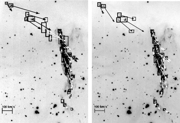
Figure 5. Proper motions of the HH 110 knots calculated from the Hα (left) and [S ii] (right) images. The underlying images were obtained with the Subaru Telescope. The boxes from which the vector originates represent the regions over which the 2D cross-correlation function was calculated. The boxes around the tips of the vectors represent the estimated errors of the proper motions. North is up and the east is left.
Download figure:
Standard image High-resolution imageThe proper motion measurements (Table 3) obtained from the Hα and [S ii] images in general agree within ∼30%. The HH 270 knots show larger proper motions that range between 91 km s−1 (knot E) and 293 km s−1 (knot D). The latter value was obtained from the Hα images, while the value obtained from the [S ii] images for the same knot is 184 km s−1. The proper motions of the HH 110 knots have values between 10 km s−1 (knot S) and 115 km s−1 (knot P'). The values obtained from the [S ii] images are somewhat different from those obtained from the Hα images. This is most noticeable in the case of knots S (10 km s−1 in Hα, 45 km s−1 in [S ii]) and U (15 km s−1 and 50 km s−1). The P.A.s of the proper motion vectors of the knots of the HH 110 jet vary from 160° (knot B) to 266° (knot U). The knots of the HH 270 jet exhibit proper motion vectors with P.A.s between 215° (knot E) and 263° (knot Z3).
The proper motion vectors of the southernmost knots of the HH 110 jet exhibit some interesting features. The projected velocities of knots R'–V range between 10 km s−1 and 48 km s−1 and are therefore much smaller than the velocities of the rest of the knots. The HH 110 knots from P' to U are positioned along a sinuous wiggle and their proper motion vectors point tangentially along the wiggle.
The HST images have enabled us for the first time to resolve some knots into substructures and to measure proper motions for 49 of them (Figures 6 and 7 and Table 4). We have measured the velocity dispersion in the HH 110 knots that show three or more substructures: A, C, E, H, I, J, and O. The results are presented in Table 5, where Column 1 shows the name of knot, Column 2 is the number of the substructures in each knot observed in the HST images, Column 3 is the average P.A., and Column 4 is the average projected velocity of the substructures in each of the knots, Columns 5 and 6 give the velocity and P.A. dispersions in each knot, and in Columns 7 and 8 there are estimated errors of the measurements of the velocity and P.A. We examine the HH 110A knot in more detail, since it is positioned close to the point of impact of the HH 270 jet (see Figure 7). We find it to have three substructures that exhibit very different proper motions. The head of the knot consists of two substructures of which the western one propagates faster (74 km s−1) and with a P.A. 261° and the eastern structure is slower with a velocity of 60 km s−1 and P.A. of 209°. These P.A.s coincide well with the angles of the axes of the HH 270 (240°) and HH 110 (194°) flows. The third substructure of the HH 110A knot is its neck, which starts as a narrow, 14 wide funnel that gradually widens at an approximately constant half-opening angle of 8° out to 72'' south of knot A. It exhibits a proper motion velocity of 14 km s−1 and P.A. of 175°.
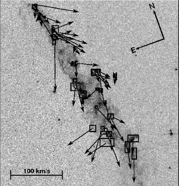
Figure 6. Proper motions of the HH 110 knots measured from the HST Hα images. The arrows in the top right corners show the orientation of the image.
Download figure:
Standard image High-resolution image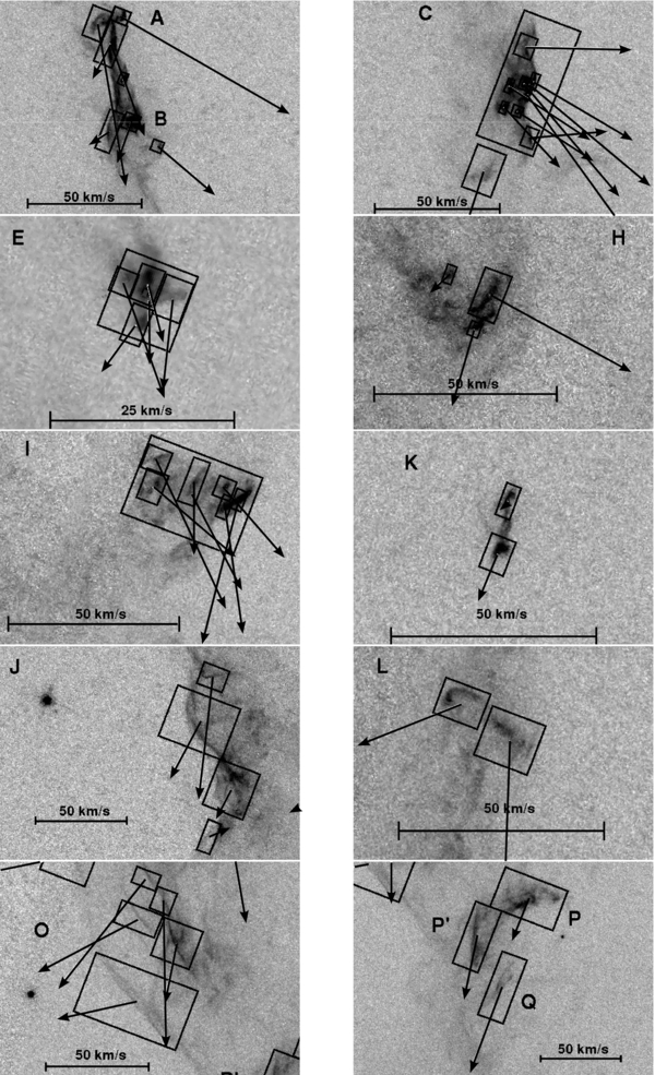
Figure 7. Proper motions of the substructures of the individual knots obtained from the HST images.
Download figure:
Standard image High-resolution imageTable 4. Results of the Observations made with the HST in the Hα Emission Line: Velocities and Angles
| Knot | v | P.A. | Knot | v | P.A. |
|---|---|---|---|---|---|
| (km s−1) | (°) | (km s−1) | (°) | ||
| A | 69 | 209 | J | 65 | 194 |
| 85 | 261 | 34 | 171 | ||
| 16 | 175 | 17 | 174 | ||
| B | 26 | 216 | 12 | 321 | |
| 17 | 183 | K | 1 | 122 | |
| 30 | 252 | 12 | 179 | ||
| 10 | 142 | L | 28 | 133 | |
| C | 42 | 246 | 32 | 194 | |
| 56 | 243 | M | 56 | 197 | |
| 60 | 239 | 53 | 222 | ||
| 33 | 243 | N | 51 | 211 | |
| 36 | 260 | 27 | 235 | ||
| 47 | 259 | O | 59 | 134 | |
| 31 | 297 | 63 | 160 | ||
| 39 | 283 | 68 | 201 | ||
| 89 | 183 | 28 | 188 | ||
| E | 6 | 166 | 52 | 131 | |
| 14 | 213 | 44 | 114 | ||
| 7 | 222 | P | 39 | 189 | |
| 12 | 195 | P' | 27 | 178 | |
| H | 6 | 165 | Q | 56 | 179 |
| 41 | 259 | ||||
| 21 | 185 | ||||
| I | 48 | 231 | |||
| 31 | 250 | ||||
| 20 | 211 | ||||
| 27 | 239 | ||||
| 33 | 205 | ||||
| 35 | 208 |
Download table as: ASCIITypeset image
Table 5. Velocity Dispersion in Knots
| Knot | No. of | 〈P.A.〉 | 〈v〉 | σP.A. | σv | σ'P.A. | σ'v |
|---|---|---|---|---|---|---|---|
| Substructures | (°) | (km s−1) | (°) | (km s−1) | (°) | (km s−1) | |
| A | 3 | 215 | 57 | 43 | 36 | 4 | 2 |
| B | 4 | 198 | 21 | 47 | 9 | 3 | 4 |
| C | 9 | 250 | 48 | 32 | 18 | 14 | 4 |
| E | 4 | 199 | 10 | 25 | 4 | 11 | 13 |
| H | 3 | 203 | 23 | 50 | 18 | 1 | 8 |
| I | 6 | 224 | 32 | 19 | 9 | 6 | 8 |
| J | 4 | 215 | 32 | 71 | 24 | 1 | 1 |
| O | 6 | 155 | 52 | 34 | 15 | 8 | 10 |
Download table as: ASCIITypeset image
We determine the level of turbulence in the HH 110 jet from the HST images. As a measurement of the level of turbulence within knots, we use dispersions σv and σP.A. of the proper motions of the substructures that belong to a certain knot, which are calculated as
Here, N is the number of substructures within each knot. 〈v〉 and 〈P.A.〉 are the average values of velocity and P.A. of the proper motion vectors of substructures that belong to the same knot. Next we compare σv and σP.A. with the estimated errors of our measurements. These errors appear mainly due to the fact that HH knots are not sharply delimited objects but are extended features that in the images gradually blend with the background. When cross-correlation technique is applied, one chooses the area in the images that is to be included in the calculation. Sometimes parts of the knots may be unintentionally excluded and some background features, which are not part of the knots, may be included. These areas tend to be slightly different each time this analysis is performed and this influences the calculated proper motion vectors. In order to estimate the errors, we measure proper motions of the HH 110 knots five times, each time slightly changing the sizes and shapes of the correlation boxes. We average the measurements and calculate the errors (σ'v and σ'P.A.) which are given in Table 5.
The P.A. dispersion of knots varies from 19° (knot I) to 71° (knot J). The projected velocity dispersion of the knots is between 4 km s−1 (knot E) and 36 km s−1 (knot A). The ratio σv/〈v〉 ranges between 0.28 (knot O) and 0.77 (knot J). The estimated error σ'v is largest in the case of knots E and O. The ratio σv/σ'v is 0.3 for knot E while for all other knots it is above 1. It follows that the values of σv and σP.A. are not due to the measurement errors.
4. DISCUSSION
A comparison of the [S ii] and Hα emissions in the HH 110 jet reveals that the level of excitation of different parts of the jet varies. The two emissions generally do not coincide spatially (Figure 4). The HH 110 jet can be described as having three distinct components that exhibit different emission properties: the eastern rim, the knots, and the faint gas that surrounds the knots.
By calculating the [S ii]/Hα ratio, we can determine the level of excitation of HH knots and other features. Their excitation depends on the velocity with respect to the surrounding gas. Predictions of emission line ratios as a function of shock velocity were calculated analytically by Hartigan et al. (1987) by using planar and bow shock models. Raga et al. (1996) presented a compilation of optical spectrometry of HH objects. Observations were compared to the Hartigan et al. (1987) models. It was found that most emission line ratios agree with plane shock models, the exception being the [S ii] λ (6717+6731)/Hα ratio. Raga et al. (1996) also suggested a division into high-, intermediate-, and low-excitation spectra, depending on the [O iii] λ 5007/Hβ and [S ii] λ (6717+6731)/Hα ratios. Kajdič et al. (2006) performed gasdynamic simulations of HH jets with variable ejection velocities. The authors calculated predictions for various emission line ratios for successive knots along the jets, which correspond to internal working surfaces. Different amplitudes of velocity variability and jet densities were used. In the case of the [S ii] λ(6717+6731)/Hα emission ratio, it was found to decrease with increasing amplitude of the velocity variability, but to increase with density.
In our images, the difference between the emission of the [S ii] and Hα spectral lines is most notable in the jet's eastern rim, which in Hα images extends between the knots C and P'. It is well defined and exhibits a filamentary structure. This rim can barely be seen in the [S ii] images (see Figure 1). The [S ii]/Hα emission ratio in the rim is ∼0.1, which means that it exhibits a high- or intermediate-excitation spectrum. It is the feature with highest excitation level in the HH 110 jet. The rim's width and brightness decrease from north to south.
The second component is the knots in the jet. The [S ii]/Hα emission ratio varies strongly from knot to knot and even between different parts of the same knot. The [S ii]/Hα emission ratio remains constant in the region between the knots A and P' with the exception of knots E and G which exhibit larger values. These values are similar to those measured for knots Q to V.
We find that most of the HH 110 and HH 270 knots in our sample have high- or intermediate-excitation spectra with [S ii]/Hα < 1.5 (see Raga et al. 1996). The exceptions are the HH 110 knots G, Q, R, and partially E, H, M, N, and T. By comparing knot spectra to Kajdič et al. (2006) results, we can estimate that they correspond to relative velocities of ⩽50 km s−1 with respect to the surrounding gas. This of course also depends on other parameters in the jet, such as density and temperature.
The third component of the HH 110 jet is the faint diffuse emission that surrounds the knots. The emission line ratio of this gas slowly increases in the north–south direction between knots A and Q.
Proper motion measurements obtained from the ground-based observations agree well with the measurements from the literature (Reipurth et al. 1996; López et al. 2005). Here, we discuss nine previously unidentified knots that belong to either HH 110 (knots P', R', T, U, and V) or to the HH 270 jet (knots Z1, Z2, Z3, and Z4). Their coordinates are given in Table 2.
The axis defined by the positions of knots Z1, Z2, Z3, and Z4 is oriented differently than the axis defined by the rest of the HH 270 knots (Reipurth et al. 1996; Choi & Tang 2006). The P.A. of the axis of the Z1–Z4 knots is ∼210°, while the P.A. of the axis of the main HH 270 flow is ∼240°. The average directions of motion of both groups of objects are much more similar (∼249° and ∼240°). This suggests that the direction of ejection of HH 270 changed at least once in the past. It is not unlikely that similar changes occurred more than once, in the more distant past, perhaps due to a precession of the HH 270 axis. If so, at different times in the past, HH 270 was colliding with different parts of the molecular cloud core. Since the cloud exhibits irregular structure in 13CO (1–0) maps (Reipurth et al. 1996; Choi & Tang 2006) and in NH3 (J, K) = (1, 1) and (J, K) = (2, 2) lines (Sepúlveda et al. 2011), the angle at which the HH 270 jet was colliding with the molecular cloud in the past was also subject to changes. As a consequence the direction of propagation of the deflected HH 110 jet varied in the past, possibly producing the HH 110 jet.
The southernmost part of the HH 110 jet (knots R–V) shows a much larger wiggle than the rest of the jet. It is interesting that the proper motion vectors of these knots point along the imaginary curve that passes through these knots. Here, we consider various possibilities for the formation of this wiggle.
It could be that the precession of the axis of the HH 270 jet is responsible for the wiggle. Alternatively, the large molecular flow from IRAS 05487+0255 detected by Reipurth & Olberg (1991) and visible in our [S ii] images (HH 451, see Section 5) could push parts of the HH 110 jet from their original direction of propagation. In both cases we could account for the large wiggle of the jet, but could not answer the question of why the proper motion vectors of knots T–V point along the wiggle. So some other explanation should be looked for.
We also consider the possible role of magnetic fields in curving the HH 110 jet. Todo et al. (1993) presented three-dimensional MHD simulations of young stellar object jets. In their work, the authors assumed the existence of an ambient large-scale magnetic field that is helically twisted by the rotation of the protostar and the protostellar disk. This causes a helical kink instability to occur and the jet obtains a helical structure, which in projection is seen as wiggling. However, the amplitude of the wiggles in their simulations seems to be much smaller than that of the southern wiggle of the HH 110 jet. Also, since the HH 110 jet is most likely a deflected jet, and therefore it has no driving source, it is not clear where the helically twisted magnetic field would originate from. This makes a helical kink instability an unlikely candidate for the cause of the wiggled structure of the HH 110 jet.
The one possibility that we cannot eliminate is that the southern wiggle is caused by a Kelvin–Helmholtz (K-H) instability. It has been shown in the past (see, for example, Stone et al. 1997; Hardee & Stone 1997) that asymmetric modes of the K-H instability in supersonic (with Mach numbers up to 20) radiatively cooling jets can affect their structure and evolution. The sinusoidal asymmetric surface waves can perturb and even disrupt jets. The distance along their axis at which this happens depends, among other things, on their Mach numbers. Jets with higher Mach numbers propagate farther without being disrupted. Also, K-H instabilities can be responsible for forming some of the dense knots in these flows. Two scenarios for this have been proposed by Stone et al. (1997): (1) the jets sweep up the ambient gas by large-amplitude oscillations caused by the surface waves or disruption of the jets and (2) when in a nonlinear regime, the body waves internal to the jets form shocks inside them and strong cooling of the post-shock gas can result in condensation of dense knots.
If the K-H instability is indeed responsible for the wiggly structure of HH 110 and some of its southernmost knots, then the proper motions of these knots would consist of their propagation along the jet's axis and of the displacement of the wiggles themselves. This would broadly explain the orientation of the proper motion vectors of the southernmost HH 110 knots. Also, if these knots are due to the strong entrainment of ambient gas and/or form due to internal shocks followed by strong cooling, then this could account for their observed high [S ii]/Hα ratios.
The observations made with the HST enable us to resolve the individual HH 110 knots into smaller structures and to measure their proper motions. We measured proper motions for 49 such structures. We are able to resolve eight knots into three or more substructures. For these knots we calculate the velocity and direction dispersion within them. These dispersions seem to be much greater than the estimated measurement errors. The values of σv and σP.A. within the knots are comparable to the average values of the velocity and P.A. there. This means that the HH 110 knots are highly turbulent, as might be expected from the jet/cloud collision hypothesis.
In the case of the HH 110A knot, we find that it has a three-component structure. Two of the components form the head of the knot. The western component is propagating in a direction that coincides with the axis of the HH 270 flow. The eastern component propagates in the direction of the axis of the HH 110 flow. The projected velocities of the two components also agree with the calculated velocities of knots in each jet. The third component of the HH 110A knot is its neck, whose proper motion vector points toward the southeast. The neck forms a part of a funnel-like structure that extends all the way to the knot B and opens up with an almost constant opening angle.
The proper motions of some knots (P, Q, but especially K) obtained from the HST images are very different from the ones obtained by the ground-based telescopes. In the case of knot K, additional measurements have been carried out but with similar outcomes. The reason for this could lie in the time elapsed between the ground-based images, which is ∼15 years. It may be large enough for changes of brightness of parts of the knots to influence the proper motion measurements.
5. NEW HH OBJECTS IN THE L1617 REGION
The Hα and [S ii] images obtained at the Subaru telescope cover a large area surrounding the HH 110 flow and the nearby HH 111 jet (Reipurth 1989), and we have searched for additional new HH objects in this region. Figure 8 (top) shows an excerpt from the Hα Subaru image. The HH 110, HH 111, and HH 270 jets are prominently visible. Several more HH objects are seen, which are discussed in the following paragraphs. The bottom image in the Figure 8 shows the same region as the top image but contains labels and indications of the three principal flow axes in the region, as discussed below.

Figure 8. Top: an excerpt from the Hα Subaru image showing the region surrounding the HH 110 and the HH 111 jets. Besides the already known HH flows, there are several newly discovered objects: HH 1032, HH 1033, HH 1034, and HH 1035. Bottom: the same region but with labels and indications of three principal flow axes in the region.
Download figure:
Standard image High-resolution imageImmediately to the west of HH 110 is the major molecular outflow that arises in IRAS 05487+0255. As mentioned in Section 4, the deep Subaru images reveal a chain of faint knots centered in what appears to be an outflow cavity in the cloud core along the molecular outflow axis. We designate these knots HH 451 A, B, C, and list their coordinates in Table 2. We note that the isolated knot HH 110K lies along the well-defined axis of the HH 451 flow, and a likely better designation for this knot would be HH 451C. Two young stars, IRS 1 and 2, have been found at optical and near-infrared wavelengths (Reipurth & Olberg 1991; Davis et al. 1994; Garnavich et al. 1997), in the radio continuum (Rodríguez et al. 1998), and with Spitzer (Hartigan et al. 2009). The IRAS source 05487+0255 is likely to be a blend of several of these sources, but dominated by IRS 2.
Noriega-Crespo et al. (2002) found two HH objects, HH 490 and HH 491, in the L1617 region. HH 490 is about 4 arcmin south of HH 110, and HH 491 is at a similar distance north of HH 110. These are likely to be more distant bow shocks related to the outflow activity associated with IRAS 05487+0255 and the HH 451 flow. HH 490 is well resolved in the Subaru images, where it is seen as large, complex group of knots.
Another previously known object is HH 112, found by Reipurth & Olberg (1991), located northeast of the HH 270 flow and lying on the very northern edge of the Hα image in Figure 8.
The Subaru images show several new HH objects in the region, which we here label HH 1032, 1033, 1034, and 1035. Their locations are marked in Figure 8 (bottom), Figure 9, and Figure 10, and coordinates are given in Table 2. Figure 9 shows an archival Spitzer H2 (4.5 μm) image (PI: Noriega-Crespo) obtained on 2005 March 25, which demonstrates that many of the HH objects in the region are also emitting in H2, and that there are a number of additional knots only seen in H2. Figure 10 combines the Hα, [S ii], and H2 images into a color image of the region.

Figure 9. Infrared molecular hydrogen image showing approximately the same region as Figure 8.
Download figure:
Standard image High-resolution image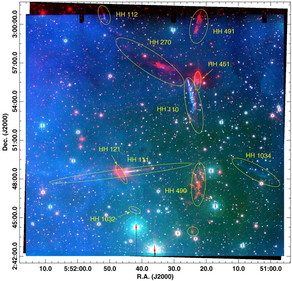
Figure 10. This color image is a combination of Hα, [S ii], and H2 images.
Download figure:
Standard image High-resolution image
HH 1032 is a small linear shock feature located precisely south of the prominent HH 111 jet, and consisting of seven or eight knots. The Subaru images are so deep that the faint glow from the photoionized skin of the molecular clouds in the area is seen. No cloud, however, is seen in immediate connection with the HH 1032 jet, nor does the large number of background stars suggest the presence of an obscuring mass near the jet. In contrast, the massive cloud core that hides the source of the HH 111 jet is readily visible in the figures. It is therefore likely that HH 1032 is a little, shocked filament of an outflow from the binary source of the HH 111 flow. In the infrared, the HH 111 core shows not only the prominent HH 111 jet, but also a shocked outflow that emanates approximately north–south from the HH 111 binary source (Gredel & Reipurth 1993, 1994), with the southern lobe pointing toward HH 1032.
Further to the southwest we find a compact, rather prominent, shock, which we here label as HH 1033. The origin of this shock is unclear, it is approximately aligned with the HH 110 flow axis and might be related to this flow, but proper motions are required to identify the source region.
Finally, we find two more diffuse objects with a fainter surface brightness. One, which we label as HH 1034, is a several arcminute long filamentary shock that lies close to the well-defined axis of the HH 111 jet. It is, however, at a rather large angle to the HH 111 jet axis, and is very unlikely to be associated with this flow. Further to the west we find another diffuse nebula, here labeled as HH 1035, which in principle could be related to HH 1034. In fact, if one draws a line from the distant HH 112 through HH 270, one arrives at HH 1034 and 1035, suggesting that these objects could form part of a giant, diffuse bow shock from the HH 270 source.
6. AN ALTERNATIVE INTERPRETATION
When examining the wide-field images in Figures 8–10, it is striking that HH 110 and HH 112 are approximately point symmetric around the HH 270 driving source. They may represent opposite ends of an S-symmetric outflow due to a precessing, presumably binary, source. The orientation of HH 110 could then be, at least in part, due to precession of the HH 270 source. Additionally, the curious structure of HH 110 with an undulating, sharp eastern border, and Hα-strong edge seen in Figure 4 would find a natural explanation if it is a kind of sideways bow shock as the HH 110 flow is bent southward additionally by the HH 451 flow. HH 110 could then be shaped not by a flow–cloud collision, but by a flow–flow collision.
In this scenario, the diffuse HH 1034/1035 objects form a bow shock that passed unimpeded to its current location from an origin in the HH 270 source, possibly because the HH 451 flow was either inactive at the time, or had not yet started.
The discovery of further HH objects in this region testifies to the complexity of star formation here. The number of shocks is so large that the flows reach the limit of confusion. A study identifying all young stars in the region, combined with future proper motion measurements, is required to identify with certainty the origin of these new HH flows. This in turn will cast light on the mechanism that produces the enigmatic HH 110 flow, whether a flow–cloud collision or a flow–flow collision.
7. CONCLUSIONS
A comparison of [S ii] and Hα intensities shows that the HH 110 jet is composed of three components. The first is the jet's eastern rim that roughly extends between knots B and P'. This rim exhibits the highest excitation level in the HH 110 jet. It is well visible in the Hα images, but is practically absent in the [S ii] images. The rim becomes fainter for the more southern regions and disappears beyond the knot P'. The second component of the HH 110 jet is its knots. The third component is the faint emission that surrounds the knots, which is less excited than the knots themselves.
The proper motion measurements of the HH 110/270 system obtained from the ground-based telescopes agree well with the previous results from Reipurth et al. (1996) and López et al. (2005). We label several previously unidentified knots and measure their proper motions. In the case of the HH 270 jet we identify four new knots and also measure their proper motions. Based on the positions of these knots (HH 270 Z1, Z2, Z3, and Z4), we conclude that the HH 270 jet axis has changed its direction at some time in the past.
HH 110 shows a strong wiggle in its southernmost parts. The proper motion vectors of knots positioned along the wiggle have directions tangential to it. One explanation that we cannot eliminate is that the wiggle is caused by a K-H instability in the southern regions of the HH 110 jet but more work has to be done in order to investigate this possibility.
The HST images enabled us to resolve some of the HH 110 knots into multiple components. We resolve 15 of the previously known knots into two or more substructures. In total we measured proper motions for 49 substructures. For eight of the knots that show three or more components, we calculate the dispersion of the projected velocity and propagation angle of the components within them. We compare these results with the estimated measurement errors. The dispersions are much larger than the errors and represent a substantial fraction of the average values of velocity in each knot, which points to the highly turbulent nature of the HH 110 jet.
Our findings on kinematics and physical conditions of the HH 110/270 system are consistent with those from the literature (López et al. 2005, 2010; Riera et al. 2003a, 2003b; Hartigan et al. 2009). We attribute the peculiar structure and shape of the HH 110 jet to the interaction of the HH 270 jet, whose characteristics (ejection velocity and flow axis) vary with time, with a nearby molecular cloud core. Further observational and theoretical work will be needed in order to fully explain the nature of the HH 110/270 system.
Shocks within the nearby molecular flow discovered by Reipurth et al. (1996) can be seen in our Subaru images and we label this flow as HH 451. It is relatively bright in [S ii], which reveals its low-excitation nature. Several other HH objects are seen in our deep Subaru images, but their origin is unclear and additional observations will be required to identify their driving sources.
When examining the large-scale structure of the outflows in the region, it becomes clear that HH 110 and the previously known HH 112 may be opposite components in a S-symmetric outflow from the HH 270 driving source. If so, this might cast some doubt on the flow–cloud collision interpretation. As an alternative, HH 110 may instead get at least part of its curious morphology from a flow–flow collision, where HH 110 is overrun by the HH 451 flow moving southward from the IRAS 05487+0255 source. Further work is required to choose between these two interpretations.
The authors thank the referee William J. Henney for his very useful comments which improved the paper. P.K. acknowledges the Dirección General de Estudios de Posgrado of the UNAM for a scholarship supporting his graduate studies and CONACyT and DGAPA for the posdoc grants. B.R. acknowledges support from NSF grant AST0407005, and from the National Aeronautics and Space Administration through the NASA Astrobiology Institute under Cooperative Agreement No. NNA09DA77A issued through the Office of Space Science. Based in part on data collected at the Subaru Telescope, which is operated by the National Astronomical Observatory of Japan (NAOJ). Based on observations taken under program GO-9901 with the NASA/ESA Hubble Space Telescope obtained at the Space Telescope Science Institute, which is operated by the Association of Universities for Research in Astronomy, Inc., under NASA contract NAS5-26555. A.R. acknowledges support from the CONACyT grants 61547, 101356, and 101975.
Facilities: Subaru (Suprime-Cam) - Subaru Telescope, HST (ACS) - Hubble Space Telescope satellite, NTT (EMMI) - New Techology Telescope