


ABSTRACT
We have begun the ExploreNEOs project in which we observe some 700 Near-Earth Objects (NEOs) at 3.6 and 4.5 μm with the Spitzer Space Telescope in its Warm Spitzer mode. From these measurements and catalog optical photometry we derive albedos and diameters of the observed targets. The overall goal of our ExploreNEOs program is to study the history of near-Earth space by deriving the physical properties of a large number of NEOs. In this paper, we describe both the scientific and technical construction of our ExploreNEOs program. We present our observational, photometric, and thermal modeling techniques. We present results from the first 101 targets observed in this program. We find that the distribution of albedos in this first sample is quite broad, probably indicating a wide range of compositions within the NEO population. Many objects smaller than 1 km have high albedos (≳0.35), but few objects larger than 1 km have high albedos. This result is consistent with the idea that these larger objects are collisionally older, and therefore possess surfaces that are more space weathered and therefore darker, or are not subject to other surface rejuvenating events as frequently as smaller NEOs.
Export citation and abstract BibTeX RIS
1. INTRODUCTION
1.1. Near-Earth Objects
The majority of Near-Earth Objects (NEOs) originated in collisions between bodies in the main asteroid belt and have found their way into near-Earth space via complex dynamical interactions. This transport of material from the main belt into the inner solar system has shaped the histories of the terrestrial planets. Together with comets, NEOs have delivered materials such as water and organics essential for the development of life, and they offer insight into both the past and future of life on Earth. The close match between the distribution of small NEOs and the lunar crater record (Strom et al. 2005) demonstrates that impacts of objects from near-Earth space are common.
The NEAR-Shoemaker and Hayabusa space missions to NEOs returned a wealth of information on two very different examples of our near-Earth neighbors, and other NEO space missions are under study. However, despite their scientific importance, key characteristics of the NEO population—such as the size distribution, mix of albedos and mineralogies, and contributions from so-called dead or dormant comets—remain largely unexplored, especially in the size range below 1 km (Stuart & Binzel 2004). Critically, recent evidence (Section 2.1.1) suggests that the size distribution of NEOs may undergo a transition at ∼1 km, and that the smaller bodies may record fundamental physical processes that are presently occurring in the solar system but not understood.
While the rate of discovery of NEOs has risen dramatically in recent years, efforts to understand the physical characteristics of these objects lag far behind. At present there are almost 7000 NEOs known. The WISE mission will discover hundreds of NEOs (Mainzer et al. 2006, 2010), and the Pan-STARRS program is likely to increase the number of known NEOs to ∼10,000 (Kaiser 2004). However, the number of NEOs with measured physical properties (albedo, diameter, rough composition) is less than 100 (e.g., Wolters et al. 2008, and references therein). Almost 99% of all NEOs remain essentially uncharacterized.
1.2. Warm Spitzer
The Spitzer Space Telescope (Werner et al. 2004) was launched in 2003 August, and carried out more than 5.5 years of cryogenic observations at 3.6–160 μm. On 2009 May 15, the onboard liquid helium cryogen ran out, making additional long wavelength observations impossible. However, because of the thermal design of the cryogenic telescope assembly and the low thermal radiation environment of its solar orbit (Gehrz et al. 2007), the telescope and instruments are passively cooled to approximately 26 K and 28 K, respectively. This allows for continued observations at the two shortest wavelengths of 3.6 μm (CH1) and 4.5 μm (CH2) with the IRAC camera (Fazio et al. 2004). In Spring 2008, NASA approved a two-year extended "Warm Spitzer" mission whose focus would primarily be on a small number of "Exploration Science" projects of 500 hr or more. We showed in Trilling et al. (2008, hereafter T08) that Warm Spitzer could successfully be used to derive the albedos and diameters of NEOs. In late 2008, we were awarded 500 hr of Warm Spitzer time to study NEOs in the ExploreNEOs program, described here.
1.3. Results from the First 101 Targets
Our observations will be carried out between 2009 July and 2011 July. In this paper, we present a description of our overall program, including target selection, observation planning, and scheduling constraints (Section 2). We present observations and measured fluxes for the first 101 targets observed in our program (Section 3). In Section 4, we describe the thermal models that we use to generate derived albedos and diameters from measured fluxes. We then describe results from the first 101 targets in our program (Section 5). Finally, we describe future directions for this project in Section 6. This paper is intended to serve as a global reference for all subsequent papers produced from the ExploreNEOs project. In particular, Section 2 (program definition), Section 3 (observations and flux measurements), and Section 4 (thermal modeling) apply not just to these first 101 targets, but to the entire project and to future papers.
2. EXPLORENEOS: THE WARM SPITZER NEO SURVEY
2.1. Science Goals
The primary science goal of the ExploreNEOs program is to explore the history of near-Earth space. We do this by studying both the global characteristics of the NEO population and the physical properties of individual objects.
2.1.1. The Size Distribution of Small NEOs
The size distribution of a population of small bodies records the evolution of that population. Most NEOs are remnants of main-belt asteroids that have reached their current location via the following sequence of events: (1) asteroids collide in the main belt and create fragments, (2) the fragments drift in semimajor axis across the main belt over hundreds of millions of years by the sunlight-driven non-gravitational thermal force called the Yarkovsky effect, and (3) they eventually reach chaotic resonances produced by planetary perturbations that can push them out of the main belt and into the terrestrial planet region (Bottke et al. 2006). The NEO population is also comprised of numerous dormant and active Jupiter-family comets, many of which originated in the Transneptunian region (Bottke et al. 2002). In much the same way that rocks in a streambed suggest the nature of events upstream, the NEO population provides us with critical clues that can tell us about the nature and evolution of the source populations (here, the main belt and Kuiper Belt).
Recent work suggests that the orbital and size distributions of NEOs may change dramatically from kilometer-sized bodies to subkilometer bodies. The evidence comes from a range of sources. (1) New work shows that the thermal spin-up mechanism called YORP causes many small NEOs to shed large amounts of mass over timescales much shorter than their dynamical lifetime (e.g., Bottke et al. 2006; Walsh et al. 2008), thus modifying the size distribution of NEOs. (2) A paucity of observed small comets as well as a lack of small craters on young surfaces like Europa indicates that the Jupiter-family comet population may be highly depleted in objects compared to our expectations for collisionally evolved populations (Bierhaus et al. 2005). If this is true, subkilometer comets essentially do not exist or some highly efficient (and unknown) mechanism eliminates them prior to reaching the vicinity of Jupiter (and possibly Saturn). Probes of the size and albedo distributions of subkilometer NEOs will provide critical constraints. (3) Young asteroid families residing near important main-belt resonances (e.g., 3:1 mean-motion resonance with Jupiter) may supply many more subkilometer asteroids than kilometer-sized asteroids (Vernazza et al. 2008; Nesvorný et al. 2009). Precise measurements of the size distribution of subkilometer NEOs will place strong constraints on these processes. (4) Preliminary debiased observations from Spacewatch indicates many subkilometer asteroids simply do not survive long enough to reach a < 2 AU orbits (J. Larsen 2008, private communication).
These lines of evidence suggest that the behavior and evolution of subkilometer NEOs may be very different from that of kilometer-sized NEOs. Precise measurements of the size distribution of NEOs will place important constraints on the interplay among the processes described above; at present, there is no large-scale empirical data set to serve as a benchmark against which theoretical models can be tested.
2.1.2. The Search for Dead Comets
A long-running debate concerns the fraction of the NEO population that has a cometary origin: how many NEOs are ex-comets that have exhausted all of their volatiles and now appear indistinguishable from asteroidal bodies? This question has important consequences for the history of near-Earth space as well as for the history of life on Earth, as comets carry significant volatile and organic material. Since the dynamical lifetimes of comets generally exceed their active lifetimes, there are expected to be a large number of dormant or extinct comets that are cataloged as asteroids. Fernandez et al. (2005) estimate that some 4% of all NEOs are "dead" comets, while Binzel et al. (2004) estimate that up to 20% of the NEO population may be extinct comets, after correcting for observational bias against the detection of low ("comet-like") albedo objects in the known population of NEOs. However, caution should be exercised in considering these results as they are based on small number statistics and largely exclude the size range below 1 km.
In the ExploreNEOs program, we will derive albedos for a large number of small NEOs. In doing so, we will measure the fraction that may be dead comets. Unlike optical surveys, we are quite sensitive to low albedo objects due to their larger ratios of thermally emitted to solar reflected radiation in both IRAC CH1 and CH2. Of course, most dark asteroids may not be dead comets; we will be guided by orbital parameters and dynamical considerations in identifying objects that may be of cometary origin (Figure 1). Since dead comets are dynamically linked to the outer solar system, just as most NEOs are links to the evolution of the main asteroid belt, we will be using NEOs as a probe of the evolution of the small body populations of the solar system.

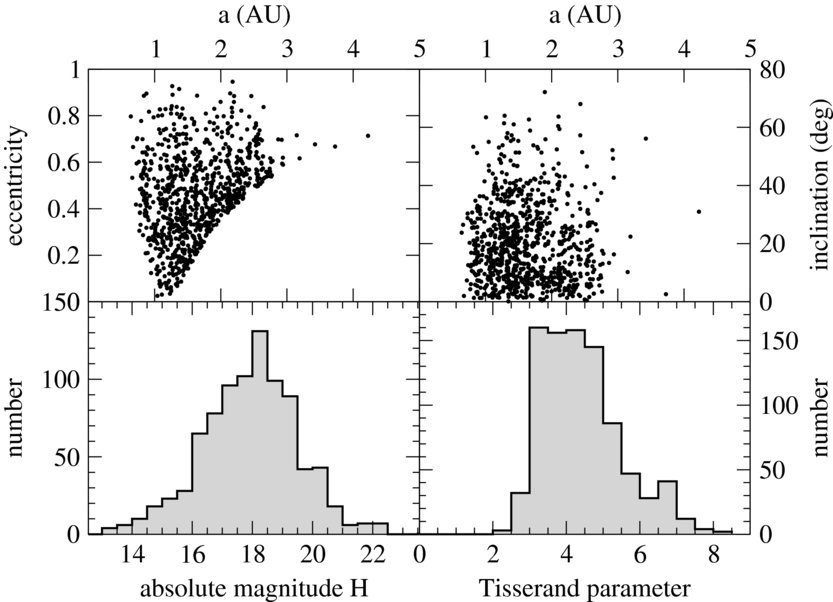
Figure 1. Our pool of target objects, showing orbital elements, solar system absolute magnitude H, and Tisserand parameter with respect to Jupiter. Some 5% of our targets have TJ < 3, suggestive of bodies that may have originated in the outer solar system.
Download figure:
Standard image High-resolution image2.1.3. NEO Origins and Compositions
The majority of NEOs are believed to be S-class asteroids, a rocky and relatively volatile poor asteroid type generally found in the inner main belt (Stuart & Binzel 2004). The majority of main-belt asteroids are C-type asteroids, more volatile and organic rich and generally found in the outer main belt (Gradie & Tedesco 1982; Carvano et al. 2010). In general, S asteroids have moderately high albedos (≳0.15) and C asteroids have low albedos (≲0.10). The interplay between the source regions, dynamical paths, and overall evolution of main-belt asteroids to NEOs is complicated (e.g., Wisdom 1982; Froeschle & Scholl 1986; Bottke et al. 2002). Measuring the albedos of a large number of NEOs will allow us to determine the relative mixing fractions of main-belt asteroids and outer solar system objects in near-Earth space.
We will also measure the albedo distribution as a function of size. As described above, the relative fractions of inner and outer solar system objects may differ for small (subkilometer) and larger (kilometer-sized) NEOs. Precise measurements of the albedo distribution as a function of size will constrain the evolution of those very small bodies.
Delbo' et al. (2003) found that the albedos for S-class (and related classes) NEOs rise from their main-belt average value of around 0.22 to greater than 0.3 for objects smaller than 500 m. Harris (2006) re-examined the trend and found that while detection bias against small dark objects may contribute, it is unlikely to be the sole explanation. Results from our Spitzer pilot study appear to confirm this trend (T08), though with small numbers and error bars which are not insignificant. Smaller objects should have statistically younger surfaces (more likely to have suffered a recent surface-refreshing event), so change in albedo with size could be an indication of space weathering processes. These processes have been studied for S types (e.g., Hapke 2001; Chapman 2004) but are much less well understood for the darker C types, for which we will derive excellent albedos (due to their darker surfaces, as described above).
2.1.4. The Physical Properties of Individual NEOs
Most airless bodies in the solar system are covered to some degree with regolith, layers of pulverized rock that are produced over time by collisions with both large and small bodies. Our Warm Spitzer NEO survey will take us into a size regime in which very little is known about asteroid regolith properties. It has been suggested, based on indirect evidence, that bodies smaller than 5 km may be nearly devoid of fine regolith (Binzel et al. 2004; Cheng 2004), but recent thermal observations apparently do not confirm this expectation (Harris et al. 2005, 2007; Delbo' et al. 2007; Mueller 2007). The small (500 m long) NEO Itokawa was visited by the Japanese spacecraft Hayabusa, and was found to have a highly varied surface, with both regolith-free regions and regions of substantial regolith. This unexpected result has greatly increased interest in the surface properties of NEOs and how they depend on an object's history. Furthermore, the presence or the absence of regolith strongly influences surface thermal inertia, which is a measure of the resistance of a material to temperature changes (e.g., diurnal cycles) and which is a key parameter in model calculations of the Yarkovsky effect, which causes gradual drifting of NEO orbits and is therefore an important dynamical effect.
While our Warm Spitzer observations will not allow us to measure thermal inertia directly, indirect information can be gained from the distribution in apparent color temperature, which is determined from the thermal flux ratio at IRAC wavelengths. The thermal flux ratio will be measured with high significance in the case of low-albedo targets, for which contamination from reflected sunlight is much reduced. We will derive the average thermal inertia of our target sample—and therefore information on the absence or the presence of regolith—from a statistical analysis of the color-temperature distribution. Delbo' et al. (2007) have used this method, using a much smaller database of ground-based observations, to determine the typical thermal inertia of ∼1 km NEOs. Our ExploreNEOs program will allow us to determine for the first time the typical thermal inertia of subkilometer NEOs. This result will be crucial for modeling the Yarkovsky effect, as the strength of the Yarkovsky effect depends sensitively on thermal inertia (e.g., Bottke et al. 2006). Additionally, understanding—and potentially mitigating—the Earth impact hazard requires detailed analysis of the thermal inertia and consequent Yarkovsky effect on NEOs (Giogini et al. 2002; Milani et al. 2009).
Perhaps 15% of NEOs are binaries (Pravec et al. 2005). While Warm Spitzer will not be able to resolve binary NEOs, thermal measurements of NEOs that are known to be binary or that turn out to be binaries will yield densities (assuming that the members of the binary share a common albedo and density), which in turn suggest compositions and internal strengths. (Reasonably high-quality orbital periods and semimajor axes are necessary to derive densities.) This is the only way to measure the internal properties of non-eclipsing asteroids short of visiting them with spacecraft. In this program, we are likely to measure fluxes for tens of NEOs that will turn out to be binaries, enabling future work that constrains the evolution of those bodies and, by proxy, the entire NEO population.
2.1.5. Impact of Our Results: The Congressional Mandate and Public Awareness
The U.S. Congress has mandated that 90% of all NEOs larger than 140 m in diameter be identified by 2020 using a combination of ground-based and space-based facilities. As discussed by the Science Definition Team report to Congress,11 this retires 90% of the hazard posed to the Earth by asteroid impacts. Thermal observations of the NEO population will allow us to derive the true NEO size distribution, which the optical surveys do not do; they measure the brightness distribution, which cannot be converted to a size distribution easily because the albedos of the NEOs are unknown. Knowledge of the size distribution is critical for estimates of the Earth impact hazard. Increased understanding of radiation forces is important both because small bodies undergo orbital evolution due to the Yarkovsky effect, but also because radiation forces have been proposed as a mitigation technique. In both cases, a more complete understanding, based on observations, is necessary.
2.2. Design of the Program
NEOs have relatively hot dayside surface temperatures (>250 K). Fluxes in IRAC CH1 and CH2 will therefore contain large thermal flux components (Figure 2). Sizes of NEOs can be derived from their thermal measurements. These size determinations can be combined with reflected light data (visible magnitudes obtained from ground-based observations) to derive albedos.
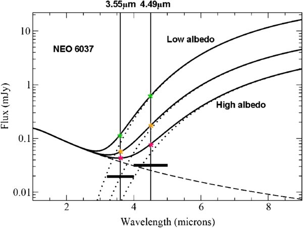
Figure 2. Spectral energy distribution (SED) of an example NEO observed in T08 (middle solid curve, for an albedo of 0.37). Also shown are hypothetical SEDs for this object if it were to have a low albedo (pV of 0.1, top curve) or high albedo (pV of 0.6, bottom curve) with the H value held constant. The dashed curve shows the reflected light component and the dotted curves show the thermal components. The combined fluxes are given by the solid curves. The thick horizontal lines indicate the approximate sensitivity levels at the Warm Spitzer wavelengths applicable to our program. The stars indicate the points on the combined flux curves at which the fluxes are measured; the vertical distances between these points and the dotted lines indicate the extent to which reflected sunlight contributes to the flux measurements. The problem increases with increasing albedo. The method for correcting for reflected sunlight is described in Section 3.
Download figure:
Standard image High-resolution image2.2.1. Sample Selection and Subsamples
Our target selection process is as follows. We began with the list of all known NEOs as of 2008 July (∼5000 bodies). For each of these, we calculated the dates when the target is within the Spitzer visibility zone (solar elongations 82 5–120°). We further culled to retain only those objects with small positional uncertainties (<150'') as seen by Spitzer during those times to ensure that these targets will fall within the IRAC field of view. We applied a cut to ensure that no object is moving faster than the Spitzer tracking rate of 1 arcsec s−1 (no presently known NEOs are excluded by this cut). The remaining list is our pool of targets. This pool includes NEOs that span a range of sizes, orbits, and (presumably) physical properties (Figure 1).
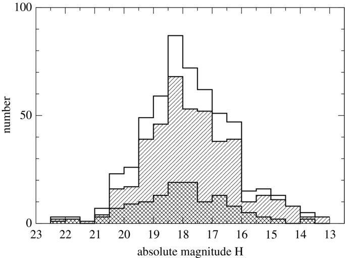
We divided these targets into two subsamples in order to maximize scientific returns and limit required telescope time. The first pool, which we call the "certain" pool (PID 60012, where the PID is the unique Spitzer Program identification number; 584 targets), contains all targets that do not have the longest exposures times (see below), as well as all targets with Tisserand parameters with respect to Jupiter less than 3.1. These low Tisserand parameter values are thought to suggest a higher likelihood of an object's origin in the outer solar system (Levison 1996), as opposed to the main asteroid belt. We use a cutoff of 3.1 instead of the nominal cutoff of 3.0 in order to be able to probe any effect completely. The second pool (PID 61013; 77 targets) contains all remaining targets with the longest integration times. Around 70% of these targets will be observed as a statistical sample. We note that because of the large variation in flux for a given NEO over its visibility window, choosing the brightest targets at any given time does not bias against targets with the largest H values (Figure 3).

Figure 3. Distribution of H (solar system absolute magnitude) for our targets. Shown here are histograms for the entire sample (tall clear histogram); all targets with tint < 2000 s (upper right to lower left hatching); and all targets with tint = 2000 s (upper left to lower right hatching). All histograms count from the bottom; that is, there are ∼50 targets in the "not-longest" (upper right to lower left) and 10 targets in the "longest" (upper left to lower right) bins at H = 17.5–18. The distributions for "not-longest" and "longest" are very similar, which means that observing fewer objects at the longest integration times does not introduce a significant bias.
Download figure:
Standard image High-resolution imageWe have three more subsamples in our ExploreNEOs program. The "ground-truth" targets (PID 61012; two targets) are NEOs that were not already included in our sample and about which we know albedo and diameter through some independent set of measurements (spacecraft, radar, etc.), and which will be used as calibrators for our larger program. We also have a sample of multi-visit targets (PID 61011; ∼10 targets), which will be observed over a range of observational geometries in order to assess systematics in our thermal modeling. Finally, we have a pool of generic targets (PID 61010; 25 targets), which are observations that are planned but whose targets are unspecified at this time. These observations will be used to observe NEOs are that have been discovered (or whose orbits have been refined) since our primary target list was fixed.
2.2.2. Observational Strategy
Since the fluxes for NEOs change dramatically on a daily basis, the most efficient way to carry out this program would be to have a different planned observation for each day of the Warm Spitzer mission, for each target, with integration times carefully customized for the predicted brightnesses. However, neither our team nor the Spitzer Science Center (SSC) could realistically deal with this explosion of candidate observations. Instead, we adopted a set of template observations with integration times of [100, 400, 1000, 2000] s per channel. We reject observations which would require integration times of more than 2000 s to reach the required signal-to-noise ratio (S/N). All generic targets are assigned the 2000 s integration time, our longest.
We set our minimum detection threshold at S/N ⩾ 15 as of 2010 June 1 (replacing the S/N ⩾ 10 requirement used prior to that date). We calculate the smallest exposure time for which a given target is visible to Spitzer with our minimum detection threshold for at least five consecutive days; this five-day window aids in scheduling our observations. Thus, a target that is bright enough to be observed with a short integration time for only a few days is assigned a longer integration time in exchange for a more generous timing constraint. This improves the overall schedulability of our program substantially while still grossly tailoring AORs to predicted target fluxes. (A Spitzer AOR is an Astronomical Observing Request—essentially, a single planned observation.) The final result is that each target is assigned a single integration time for the duration of the Warm Spitzer mission. There are [309, 149, 101, 25] targets that have integration times of [100, 400, 1000, 2000] s in PID 60012. (All AORs in the other four PIDs have 2000 s integration times.)
We use the moving cluster Astronomical Observation Template (a fixed observing pattern used by Spitzer), tracking according to the standard NAIF ephemeris. We eliminate all potential observations near the galactic plane because of background source confusion. Our dithered observations alternate between the bandpasses during the observation to reduce the relative effects of any lightcurve variations within the observing period, and to maximize the relative motion of the asteroid to help reject background sources; this technique has been validated in T08. For observations that have sufficient S/N in the individual exposures (or some binning of frames), we check for variations over the duration of the AOR.
2.2.3. Predicted Fluxes
Our flux predictions are based on the solar system absolute optical magnitude H, a measure of D2pV, as reported by Horizons. (Here D is the diameter and pV is the geometric albedo, or reflectivity). H values for NEOs are of notoriously low quality and tend to be skewed toward too bright values (Juric et al. 2002; Romanishin & Tegler 2005; Parker et al. 2008). We therefore assume an H offset (ΔH) of [0.6, 0.3, 0.0] mag for [faint, nominal, bright] fluxes, respectively. That is, we hypothesize that the nominal true magnitude of a given object is 0.3 mag fainter than the Horizons value, within a range 0.6–0.0 mag fainter than the Horizons value. Reflected light fluxes are calculated from H + ΔH together with the observing geometry and the solar flux at IRAC wavelengths. Nominally, asteroids are assumed to be 1.4 times more reflective at IRAC wavelengths than in the V band (T08; Harris et al. 2009). Thermal fluxes also depend on pV (D is determined from H and pV) and η, a model parameter that attempts to capture details of the physical properties (rotation rate, surface roughness, etc.) of the asteroid. We assumed pV = [0.4, 0.2, 0.05] for the [faintest, nominal, brightest] thermal fluxes, that is, we hypothesized that asteroid albedos are in the range 0.05–0.4 (Tedesco et al. 2002; Binzel et al. 2002). The nominal η value is determined from the solar phase angle α using the linear relation given by Wolters et al. (2008); 0.3 is [added, subtracted] for [faint, bright] fluxes to capture the scatter in the empirical relationship derived in Wolters et al.
From this range of parameters, we calculate the range of predicted fluxes in the two IRAC bands for each day of the two-year Warm Mission. The resulting thermal fluxes are convolved with the posted IRAC passbands12 to yield predicted fluxes. We then calculate the integration time required to reach the required S/N for the faintest predicted flux for each target for each day.
2.2.4. Scheduling
Each of our targets, with few exceptions, has at least one acceptable visibility window of at least five days. A few targets have no available visibility windows of five days or longer; for these we take the longest available visibility window. Since the nature of our program is that of a large sample in which individual measurements are less important than the entire suite of results, if a small number of observations fail, either through scheduling issues or data quality issues, the overall impact of this program is not affected. With ∼700 targets to observe during the two-year Warm Mission, nominally we expect to have one target observed per day, on average, and our yield to date has been slightly higher than this expected rate.
3. OBSERVATIONS AND FLUX MEASUREMENTS
We report here observations made during the period 2009 July 28 through 2009 November 4 (that is, from the IRAC warm instrument characterization, IWIC, campaign through the end of the seventh post-cryo [warm] campaign, PC007). The data were reduced using the IRACproc software (Schuster et al. 2006), which is based on the mopex routines provided by the SSC (Makovoz & Khan 2005). The Basic Calibrated Data produced by version 18.12.0 of the pipeline were used in the reduction. Mosaics of each AOR were constructed using the "moving object mode," which aligns the individual images in the rest frame of the moving target, based on its projected motion. The outlier rejection in the mosaicking process then removes or minimizes the fixed background objects in the field and any transients due to cosmic rays or array artifacts. The images are rebinned to a pixel scale of 0 8627 pixel−1 in the final mosaics. We extracted the photometry using the phot task in IRAF. The noise in the image was estimated in the region near the NEO, and the extraction used an aperture radius of 6 mosaic pixels (51762), with a sky annulus with an inner radius of 6 pixels and an outer radius of 12 pixels. These parameters are significantly smaller than the aperture size of 10 instrumental pixels (122) used in the IRAC calibration measurements (Reach et al. 2005). The smaller aperture was chosen to reduce the effects of background objects in the aperture in crowded fields where some of the NEOs were observed. In order to calibrate our NEO photometry, we extracted the photometry of IRAC calibration stars observed in the same campaigns as our NEO observations, at the same detector temperature and bias settings. Our zero points in channels 1 and 2 were then adjusted to make the standard star magnitudes match those reported by Reach et al. (2005). For the observations taken after the final IRAC warm mission biases and temperatures were set on 2009 September 24, the zero points used are 17.864 and 17.449 mag for the 3.6 and 4.5 μm bands, respectively. The measured fluxes and associated errors are reported in Table 1.
Table 1. Target Information and Results
| Target | PID | AOR | Date Obs. | F3.6 | F4.5 | r | Δ | Phase | pV | D | η | H | Notes |
|---|---|---|---|---|---|---|---|---|---|---|---|---|---|
| (UT) | (μJy) | (μJy) | (AU) | (AU) | (deg) | (km) | (mag) | ||||||
| 433 Eros 1898 DQ | 60012 | 32648448 | 2009 Aug 25T06:16:48 | 13990 ± 110 | 40230 ± 200 | 1.702 | 1.218 | 36.50 | 0.06 | 31.93 | 1.39 | 11.2 | 1 |
| 1863 Antinous 1948 EA | 60012 | 32698112 | 2009 Sep 02T12:50:32 | 5422 ± 71 | 21070 ± 130 | 1.024 | 0.240 | 83.28 | 0.10 | 3.23 | 1.99 | 15.5 | |
| 1943 Anteros 1973 EC | 60012 | 32641536 | 2009 Sep 15T00:09:48 | 189 ± 13 | 582 ± 22 | 1.548 | 0.951 | 40.17 | 0.15 | 2.43 | 1.43 | 15.8 | |
| 2100 Ra-Shalom 1978 RA | 61012 | 35304192 | 2009 Aug 27T01:22:49 | 937 ± 29 | 4841 ± 63 | 1.056 | 0.415 | 74.12 | 0.14 | 2.22 | 1.87 | 16.1 | 1 |
| 3103 Eger 1982 BB | 60012 | 32584448 | 2009 Aug 24T22:47:37 | 162 ± 12 | 243 ± 14 | 1.584 | 1.011 | 39.14 | 0.39 | 1.79 | 1.42 | 15.4 | |
| 4183 Cuno 1959 LM | 60012 | 32591104 | 2009 Aug 20T09:41:02 | 4387 ± 61 | 18420 ± 130 | 1.171 | 0.524 | 60.71 | 0.10 | 5.49 | 1.70 | 14.4 | |
| 4953 1990 MU | 60012 | 32654336 | 2009 Aug 21T00:58:18 | 16.3 ± 3.9 | 17.9 ± 4.0 | 2.667 | 2.091 | 20.61 | 0.79 | 2.26 | 1.18 | 14.1 | |
| 4957 Brucemurray 1990 XJ | 60012 | 32616448 | 2009 Aug 13T04:04:51 | 81.6 ± 8.7 | 193 ± 13 | 1.781 | 1.589 | 34.69 | 0.17 | 3.06 | 1.36 | 15.1 | |
| 5143 Heracles 1991 VL | 60012 | 32667648 | 2009 Sep 19T01:20:11 | 2211 ± 44 | 8883 ± 89 | 1.080 | 0.435 | 71.12 | 0.42 | 3.26 | 1.83 | 14.0 | |
| 5604 1992 FE | 60012 | 32598272 | 2009 Aug 06T13:52:59 | 510 ± 21 | 1868 ± 39 | 1.061 | 0.210 | 73.26 | 0.69 | 0.84 | 1.86 | 16.4 | 1 |
| 5620 Jasonwheeler 1990 OA | 60012 | 32659968 | 2009 Aug 25T07:00:35 | 258 ± 16 | 1252 ± 33 | 1.321 | 0.620 | 48.68 | 0.09 | 1.75 | 1.54 | 17.0 | |
| 5626 1991 FE | 60012 | 32574464 | 2009 Aug 21T03:23:36 | 434 ± 20 | 1209 ± 31 | 1.689 | 0.972 | 33.08 | 0.15 | 3.96 | 1.34 | 14.7 | |
| 7822 1991 CS | 60012 | 32693248 | 2009 Aug 25T04:37:42 | 141 ± 13 | 420 ± 19 | 1.122 | 0.514 | 65.61 | 0.28 | 0.83 | 1.76 | 17.4 | |
| 7888 1993 UC | 60012 | 32576768 | 2009 Aug 06T17:17:59 | 142 ± 12 | 456 ± 20 | 1.535 | 1.213 | 41.56 | 0.18 | 2.75 | 1.45 | 15.3 | |
| 8566 1996 EN | 60012 | 32651264 | 2009 Oct 17T05:43:42 | 80.3 ± 8.7 | 223 ± 14 | 1.317 | 0.963 | 50.63 | 0.28 | 1.25 | 1.57 | 16.5 | |
| 9950 ESA 1990 VB | 60012 | 32644352 | 2009 Oct 06T01:02:44 | 2386 ± 45 | 9875 ± 89 | 1.216 | 0.360 | 50.59 | 0.10 | 2.47 | 1.57 | 16.2 | |
| 10302 1989 ML | 60012 | 32642048 | 2009 Aug 21T03:09:36 | 229 ± 15 | 560 ± 22 | 1.100 | 0.152 | 56.01 | 0.49 | 0.24 | 1.64 | 19.5 | |
| 12711 1991 BB | 60012 | 32593664 | 2009 Oct 16T16:45:35 | 371 ± 19 | 1242 ± 32 | 1.172 | 0.708 | 60.28 | 0.19 | 1.94 | 1.69 | 16.0 | |
| 15745 1991 PM5 | 60012 | 32624384 | 2009 Aug 25T06:47:16 | 66.2 ± 9.3 | 209 ± 14 | 1.361 | 0.632 | 45.54 | 0.23 | 0.77 | 1.50 | 17.8 | |
| 16834 1997 WU22 | 60012 | 32666112 | 2009 Sep 06T17:43:13 | 67.1 ± 9.3 | 134 ± 12 | 1.514 | 1.225 | 42.30 | 0.40 | 1.52 | 1.46 | 15.7 | |
| 17274 2000 LC16 | 60012 | 32685824 | 2009 Aug 25T06:31:32 | 1711 ± 39 | 7533 ± 83 | 1.201 | 0.753 | 57.88 | 0.01 | 5.01 | 1.66 | 16.7 | |
| 20460 Robwhiteley 1999 LO28 | 60012 | 32597504 | 2009 Aug 20T08:56:45 | 2011 ± 42 | 8146 ± 82 | 1.239 | 0.634 | 55.40 | 0.04 | 4.57 | 1.63 | 15.7 | |
| 20826 2000 UV13 | 60012 | 32634880 | 2009 Aug 20T23:32:41 | 33.3 ± 5.5 | 31.8 ± 5.3 | 3.190 | 2.640 | 17.09 | 0.27 | 5.12 | 1.13 | 13.5 | |
| 27346 2000 DN8 | 60012 | 32587008 | 2009 Aug 22T21:19:03 | 142 ± 12 | 485 ± 21 | 1.350 | 0.997 | 48.88 | 0.19 | 1.92 | 1.54 | 16.0 | |
| 38086 Beowolf 1999 JB | IWIC | IWIC | 2009 Jul 26T00:27:03 | 26.4 ± 5.3 | 156.7 ± 4.4 | 1.187 | 0.715 | 58.64 | 0.37 | 0.72 | 1.67 | 17.4 | |
| 40329 1999 ML | 60012 | 32603648 | 2009 Sep 03T00:25:52 | 197 ± 14 | 623 ± 23 | 1.344 | 0.501 | 41.48 | 0.16 | 0.94 | 1.45 | 17.7 | |
| 42286 2001 TN41 | 61013 | 32717568 | 2009 Oct 26T23:05:59 | 24.7 ± 4.7 | 19.3 ± 4.2 | 1.961 | 1.236 | 26.92 | 1.03 | 0.69 | 1.26 | 16.4 | 1 |
| 52387 1993 OM7 | 60012 | 32558592 | 2009 Sep 01T10:12:03 | 95.1 ± 9.6 | 333 ± 17 | 1.520 | 0.727 | 35.88 | 0.09 | 1.22 | 1.38 | 17.8 | |
| 54401 2000 LM | 60012 | 32578048 | 2009 Oct 26T22:05:42 | 50.2 ± 7.0 | 118 ± 10 | 1.494 | 0.890 | 42.10 | 0.22 | 0.98 | 1.46 | 17.3 | |
| 54686 2001 DU8 | 60012 | 32586496 | 2009 Oct 29T01:20:33 | 65.8 ± 8.2 | 96.6 ± 9.3 | 1.749 | 1.019 | 31.29 | 0.34 | 1.25 | 1.32 | 16.3 | 2 |
| 55532 2001 WG2 | 60012 | 32642816 | 2009 Aug 28T01:26:05 | 285 ± 17 | 985 ± 30 | 1.223 | 0.792 | 56.28 | 0.14 | 1.96 | 1.64 | 16.3 | |
| 65679 1989 UQ | 60012 | 32638976 | 2009 Oct 15T20:50:49 | 405 ± 61 | 2264 ± 43 | 1.129 | 0.237 | 58.64 | 0.06 | 0.71 | 1.67 | 19.4 | |
| 67381 2000 OL8 | 60012 | 32635648 | 2009 Aug 25T05:03:54 | 22.6 ± 4.5 | 90.8 ± 8.7 | 1.134 | 0.381 | 63.58 | 0.25 | 0.28 | 1.74 | 19.9 | |
| 68372 2001 PM9 | 60012 | 32563968 | 2009 Aug 20T10:32:54 | 3928 ± 59 | 19610 ± 140 | 1.130 | 0.204 | 53.62 | 0.02 | 1.70 | 1.61 | 18.9 | |
| 85938 1999 DJ4 | 61013 | 32720896 | 2009 Aug 13T15:40:18 | 17.2 ± 3.9 | 62.0 ± 7.2 | 1.409 | 0.688 | 43.10 | 0.28 | 0.48 | 1.47 | 18.6 | |
| 85989 1999 JD6 | 60012 | 32661248 | 2009 Aug 31T12:59:55 | 1618 ± 37 | 8506 ± 85 | 1.261 | 0.390 | 45.22 | 0.04 | 2.39 | 1.50 | 17.1 | |
| 90367 2003 LC5 | 60012 | 32583424 | 2009 Aug 24T23:16:30 | 279 ± 16 | 1590 ± 37 | 1.391 | 0.705 | 45.06 | 0.03 | 2.39 | 1.50 | 17.7 | |
| 99799 2002 LJ3 | 60012 | 32613120 | 2009 Sep 19T22:38:45 | 125 ± 15 | 392 ± 20 | 1.238 | 0.354 | 46.18 | 0.42 | 0.49 | 1.51 | 18.1 | |
| 108519 2001 LF | 60012 | 32636160 | 2009 Aug 13T13:09:08 | 1707 ± 39 | 9686 ± 87 | 1.240 | 0.366 | 46.19 | 0.02 | 2.31 | 1.51 | 17.9 | |
| 138883 2000 YL29 | 60012 | 32592640 | 2009 Oct 15T22:49:18 | 108 ± 10 | 318 ± 17 | 1.319 | 0.902 | 50.91 | 0.19 | 1.39 | 1.57 | 16.7 | |
| 138911 2001 AE2 | 60012 | 32662272 | 2009 Aug 13T14:53:37 | 24.4 ± 4.7 | 88.8 ± 8.6 | 1.330 | 0.483 | 41.78 | 0.34 | 0.34 | 1.45 | 19.1 | |
| 138925 2001 AU43 | 60012 | 32616960 | 2009 Aug 25T03:00:42 | 535 ± 23 | 2389 ± 45 | 1.182 | 0.645 | 59.84 | 0.11 | 2.41 | 1.69 | 16.1 | |
| 138937 2001 BK16 | 60012 | 32672256 | 2009 Aug 23T12:50:06 | 87.4 ± 8.9 | 359 ± 17 | 1.182 | 0.629 | 59.86 | 0.21 | 0.92 | 1.69 | 17.5 | |
| 143651 2003 QO104 | 60012 | 32694272 | 2009 Aug 21T02:40:18 | 276 ± 42 | 1052 ± 31 | 1.402 | 0.801 | 45.93 | 0.13 | 2.31 | 1.51 | 16.0 | |
| 152637 1997 NC1 | 60012 | 32675584 | 2009 Aug 22T20:20:23 | 1344 ± 35 | 3434 ± 55 | 1.046 | 0.088 | 72.53 | 0.59 | 0.43 | 1.85 | 18.0 | |
| 153220 2000 YN29 | IWIC | IWIC | 2009 Jul 26T00:03:10 | 2877.1 ± 8.6 | 10928 ± 11 | 1.068 | 0.119 | 62.27 | 0.27 | 0.81 | 1.72 | 17.5 | |
| 159399 1998 UL1 | 60012 | 32701184 | 2009 Aug 13T06:56:16 | 46.7 ± 8.2 | 110 ± 10 | 1.502 | 1.130 | 42.84 | 0.27 | 1.24 | 1.47 | 16.6 | |
| 159402 1999 AP10 | 60012 | 32682752 | 2009 Aug 31T22:54:56 | 90 ± 10 | 278 ± 16 | 1.292 | 0.838 | 52.32 | 0.34 | 1.20 | 1.59 | 16.4 | |
| 159608 2002 AC2 | 60012 | 32590848 | 2009 Aug 25T00:11:43 | 6242 ± 75 | 27020 ± 160 | 1.108 | 0.157 | 53.63 | 0.20 | 1.51 | 1.61 | 16.5 | |
| 162195 1999 RK45 | 60012 | 32689408 | 2009 Nov 03T14:22:00 | 476 ± 21 | 1602 ± 37 | 1.088 | 0.147 | 60.85 | 0.19 | 0.39 | 1.70 | 19.5 | |
| 162483 2000 PJ5 | 60012 | 32579840 | 2009 Aug 21T02:55:14 | 287 ± 17 | 1026 ± 30 | 1.196 | 0.393 | 55.03 | 0.21 | 0.92 | 1.62 | 17.5 | |
| 163758 2003 OS13 | 60012 | 32601856 | 2009 Jul 30T15:39:01 | 17.5 ± 3.9 | 45.3 ± 6.1 | 1.538 | 0.922 | 39.88 | 0.44 | 0.66 | 1.43 | 17.4 | |
| 164201 2004 EC | 60012 | 32613888 | 2009 Jul 30T18:51:35 | 845 ± 27 | 5092 ± 66 | 1.158 | 0.560 | 61.67 | 0.12 | 2.87 | 1.71 | 15.6 | |
| 164202 2004 EW | 60012 | 32667392 | 2009 Aug 06T05:32:19 | 45.9 ± 6.2 | 135 ± 10 | 1.049 | 0.158 | 75.37 | 0.35 | 0.16 | 1.89 | 20.8 | |
| 177614 2004 HK33 | 60012 | 32569600 | 2009 Jul 30T16:25:59 | 5895 ± 71 | 22920 ± 140 | 1.057 | 0.095 | 63.88 | 0.19 | 0.93 | 1.74 | 17.6 | |
| 184990 2006 KE89 | 60012 | 32604672 | 2009 Aug 14T08:13:19 | 103 ± 11 | 371 ± 18 | 1.228 | 0.805 | 55.75 | 0.29 | 1.24 | 1.64 | 16.5 | |
| 1996 EO | 61013 | 32724992 | 2009 Sep 06T18:56:13 | 25.4 ± 4.7 | 99.3 ± 9.1 | 1.151 | 0.540 | 62.84 | 0.24 | 0.42 | 1.73 | 19.1 | |
| 1996 TY11 | 60012 | 32576256 | 2009 Sep 01T19:41:57 | 230 ± 14 | 941 ± 28 | 1.056 | 0.248 | 75.79 | 0.09 | 0.62 | 1.90 | 19.3 | |
| 1998 QE2 | 60012 | 32680960 | 2009 Sep 23T02:32:45 | 514 ± 22 | 2562 ± 46 | 1.183 | 0.728 | 59.35 | 0.06 | 2.75 | 1.68 | 16.4 | |
| 1998 SV4 | 60012 | 32625664 | 2009 Oct 06T11:24:45 | 79.3 ± 8.3 | 327 ± 16 | 1.321 | 0.530 | 46.02 | 0.20 | 0.74 | 1.51 | 18.0 | |
| 1999 TX2 | 60012 | 32564736 | 2009 Oct 26T21:29:07 | 326 ± 18 | 1299 ± 34 | 1.142 | 0.362 | 62.24 | 0.11 | 0.96 | 1.72 | 18.1 | |
| 2000 GV147 | 60012 | 32620288 | 2009 Oct 24T06:09:18 | 100 ± 10 | 337 ± 17 | 1.064 | 0.336 | 74.34 | 0.17 | 0.50 | 1.88 | 19.0 | |
| 2000 JY8 | 60012 | 32700416 | 2009 Jul 29T14:18:43 | 23.7 ± 4.8 | 100.4 ± 9.1 | 1.555 | 1.018 | 40.26 | 0.32 | 1.11 | 1.43 | 16.6 | |
| 2001 TX44 | 60012 | 32693760 | 2009 Oct 27T00:09:19 | 13.9 ± 3.5 | 37.3 ± 5.6 | 1.332 | 0.499 | 43.09 | 0.68 | 0.26 | 1.47 | 19.0 | |
| 2002 EZ2 | 60012 | 32648960 | 2009 Aug 24T11:00:05 | 14.0 ± 3.6 | 63.7 ± 7.3 | 1.241 | 0.367 | 46.42 | 0.40 | 0.21 | 1.51 | 20.0 | |
| 2002 FB6 | 60012 | 32559360 | 2009 Oct 06T12:23:39 | 264 ± 16 | 10593 ± 30 | 1.078 | 0.477 | 70.85 | 0.14 | 1.20 | 1.83 | 17.4 | |
| 2002 GO5 | 60012 | 32589056 | 2009 Oct 16T12:13:04 | 278 ± 17 | 941 ± 28 | 1.218 | 0.351 | 49.66 | 0.24 | 0.75 | 1.56 | 17.8 | |
| 2002 HF8 | 60012 | 32562432 | 2009 Aug 24T23:44:38 | 109.3 ± 9.9 | 455 ± 20 | 1.262 | 0.449 | 48.69 | 0.18 | 0.70 | 1.54 | 18.3 | |
| 2002 LS32 | 60012 | 32658688 | 2009 Aug 24T12:14:18 | 720 ± 26 | 2993 ± 51 | 1.098 | 0.163 | 58.72 | 0.29 | 0.57 | 1.67 | 18.2 | |
| 2002 LV | 60012 | 32618240 | 2009 Aug 06T05:01:48 | 456 ± 20 | 1825 ± 38 | 1.101 | 0.537 | 67.11 | 0.15 | 1.73 | 1.78 | 16.5 | |
| 2002 MQ3 | 60012 | 32682496 | 2009 Aug 22T20:35:42 | 176 ± 13 | 685 ± 24 | 1.114 | 0.290 | 64.52 | 0.32 | 0.57 | 1.75 | 18.1 | |
| 2002 NP1 | 60012 | 32556800 | 2009 Nov 04T00:16:49 | 137 ± 12 | 474 ± 20 | 1.190 | 0.479 | 58.47 | 0.25 | 0.81 | 1.67 | 17.6 | |
| 2002 OM4 | 60012 | 32668928 | 2009 Sep 19T01:41:07 | 67.2 ± 7.8 | 256 ± 15 | 1.274 | 0.772 | 53.56 | 0.30 | 1.03 | 1.61 | 16.9 | |
| 2002 QE7 | 60012 | 32637952 | 2009 Sep 23T04:42:22 | 66.2 ± 8.0 | 188 ± 13 | 1.217 | 0.329 | 47.87 | 0.34 | 0.31 | 1.53 | 19.3 | |
| 2002 TE66 | 60012 | 32696576 | 2009 Oct 30T05:22:11 | 23.6 ± 4.8 | 69.5 ± 7.7 | 1.275 | 0.668 | 53.18 | 0.39 | 0.48 | 1.60 | 18.2 | |
| 2002 UX | 60012 | 32571136 | 2009 Aug 25T03:17:58 | 157 ± 13 | 443 ± 20 | 1.285 | 0.422 | 43.82 | 0.31 | 0.65 | 1.48 | 17.8 | |
| 2003 SL5 | 60012 | 32626944 | 2009 Sep 19T23:06:20 | 289 ± 17 | 1052 ± 30 | 1.114 | 0.164 | 53.62 | 0.36 | 0.33 | 1.61 | 19.1 | |
| 2003 TJ2 | 60012 | 32632064 | 2009 Oct 29T23:14:50 | 46.5 ± 6.6 | 226 ± 14 | 1.048 | 0.369 | 76.19 | 0.23 | 0.45 | 1.90 | 18.9 | |
| 2003 TL4 | 60012 | 32567552 | 2009 Oct 16T16:59:20 | 131 ± 12 | 544 ± 22 | 1.042 | 0.185 | 79.79 | 0.22 | 0.38 | 1.95 | 19.4 | |
| 2003 UN12 | 60012 | 32628736 | 2009 Oct 06T22:51:40 | 257 ± 15 | 1506 ± 35 | 1.302 | 0.461 | 44.48 | 0.05 | 1.25 | 1.49 | 18.5 | |
| 2003 WD158 | 60012 | 32601088 | 2009 Jul 31T00:06:53 | 101 ± 11 | 402 ± 19 | 1.170 | 0.316 | 54.42 | 0.29 | 0.44 | 1.62 | 18.8 | 3 |
| 2003 WD158 | IWIC | IWIC | 2009 Jul 25T22:47:12 | 141.0 ± 5.9 | 246.0 ± 4.9 | 1.138 | 0.312 | 60.06 | 0.39 | 0.38 | 1.69 | 18.8 | 3 |
| 2003 WO7 | 60012 | 32568576 | 2009 Oct 09T15:38:14 | 225 ± 22 | 517 ± 24 | 1.237 | 0.418 | 50.83 | 0.10 | 0.68 | 1.57 | 18.9 | |
| 2004 FU64 | 60012 | 32557056 | 2009 Aug 22T20:05:13 | 175 ± 14 | 554 ± 22 | 1.169 | 0.499 | 60.79 | 0.19 | 0.91 | 1.70 | 17.6 | |
| 2004 JN13 | 60012 | 32667904 | 2009 Aug 28T21:14:08 | 429 ± 20 | 1608 ± 37 | 1.559 | 0.774 | 34.76 | 0.25 | 2.97 | 1.36 | 14.5 | |
| 2004 JX20 | 60012 | 32557824 | 2009 Jul 29T13:52:44 | 855 ± 27 | 4468 ± 58 | 1.116 | 0.314 | 64.11 | 0.01 | 1.48 | 1.74 | 19.3 | 3 |
| 2004 JX20 | IWIC | IWIC | 2009 Jul 25T23:17:44 | 1181.8 ± 2.4 | 3374.0 ± 3.4 | 1.110 | 0.301 | 64.77 | 0.02 | 1.30 | 1.75 | 19.3 | 3 |
| 2004 SB20 | 60012 | 32603904 | 2009 Oct 16T09:41:45 | 47.3 ± 7.0 | 136 ± 11 | 1.134 | 0.454 | 64.66 | 0.41 | 0.43 | 1.75 | 18.4 | |
| 2005 LY19 | 61013 | 32716288 | 2009 Oct 06T21:07:34 | 33.4 ± 4.1 | 54.9 ± 6.8 | 1.944 | 1.217 | 27.22 | 0.26 | 1.36 | 1.26 | 16.4 | |
| 2005 OU2 | 61013 | 32724224 | 2009 Oct 03T05:24:48 | 43.2 ± 6.1 | 124 ± 10 | 1.172 | 0.394 | 58.94 | 0.37 | 0.34 | 1.68 | 19.0 | |
| 2005 UH6 | 60012 | 32593920 | 2009 Oct 15T08:18:15 | 134 ± 12 | 608 ± 23 | 1.079 | 0.267 | 71.43 | 0.22 | 0.52 | 1.84 | 18.7 | |
| 2005 WC1 | 60012 | 32642560 | 2009 Aug 01T06:00:54 | 58.0 ± 6.9 | 255 ± 14 | 1.099 | 0.259 | 65.49 | 0.11 | 0.29 | 1.76 | 20.7 | |
| 2006 AD | 60012 | 32583168 | 2009 Sep 09T14:48:28 | 1500 ± 36 | 6168 ± 74 | 1.092 | 0.511 | 68.81 | 0.04 | 3.06 | 1.80 | 16.7 | |
| 2006 LF | 60012 | 32610304 | 2009 Jul 30T16:10:39 | 161 ± 13 | 711 ± 24 | 1.195 | 0.299 | 47.90 | 0.25 | 0.50 | 1.53 | 18.6 | 3 |
| 2006 LF | IWIC | IWIC | 2009 Jul 25T23:46:15 | 233.9 ± 9.0 | 899.8 ± 7.2 | 1.148 | 0.278 | 55.93 | 0.20 | 0.56 | 1.64 | 18.6 | 3 |
| 2006 MD12 | 60012 | 32600576 | 2009 Sep 01T09:43:13 | 36.4 ± 5.9 | 117 ± 10 | 1.155 | 0.332 | 58.91 | 0.43 | 0.27 | 1.68 | 19.4 | |
| 2006 NL | 60012 | 32694528 | 2009 Aug 13T14:09:58 | 24.6 ± 5.0 | 144 ± 11 | 1.106 | 0.242 | 63.63 | 0.46 | 0.22 | 1.74 | 19.7 | |
| 2006 OD7 | 60012 | 32628224 | 2009 Sep 19T12:14:38 | 195 ± 13 | 615 ± 23 | 1.113 | 0.197 | 58.96 | 0.27 | 0.33 | 1.68 | 19.5 | |
| 2006 SV19 | 60012 | 32702976 | 2009 Sep 15T16:08:48 | 109 ± 10 | 435 ± 19 | 1.166 | 0.672 | 60.97 | 0.12 | 1.06 | 1.70 | 17.8 | |
| 2006 SY5 | 60012 | 32647168 | 2009 Jul 30T18:18:27 | 31.2 ± 5.1 | 116.7 ± 9.7 | 1.093 | 0.136 | 54.07 | 0.34 | 0.09 | 1.61 | 22.1 | 1 |
| 2006 WO127 | 60012 | 32638208 | 2009 Nov 04T01:09:24 | 103 ± 11 | 350 ± 18 | 1.528 | 0.889 | 40.23 | 0.21 | 1.69 | 1.43 | 16.2 | |
| 2007 DK8 | 60012 | 32575488 | 2009 Sep 16T06:56:22 | 322 ± 17 | 1708 ± 38 | 1.173 | 0.298 | 53.68 | 0.08 | 0.79 | 1.61 | 18.9 | |
| 2007 VD12 | 60012 | 32687104 | 2009 Jul 28T14:02:11 | 30.0 ± 5.0 | 78.7 ± 8.0 | 1.232 | 0.351 | 45.88 | 0.39 | 0.22 | 1.51 | 20.0 | |
| 2007 YQ56 | 60012 | 32639488 | 2009 Aug 20T10:04:58 | 79.5 ± 8.6 | 353 ± 17 | 1.029 | 0.199 | 82.47 | 0.16 | 0.34 | 1.98 | 20.0 |
Notes. The columns are as follows: target name; Spitzer program ID; AOR, which is a unique Spitzer identifier for each observation; date and time observed, which is accurate to a few seconds at 3.6 μm and tens of seconds at 4.5 μm, and which is not corrected for light travel time; measured fluxes at 3.6 and 4.5 μm; heliocentric and Spitzer-centric distances; phase angle of observations; derived albedo and diameter, using the η value given; absolute magnitude (H), from Horizons, reported only to a single decimal place; and additional notes (if any). The η values given here represent the fixed-η solutions and are derived from the phase angle (Section 5.1). Uncertainties on individual diameter and albedo values are estimated to be 25% and 50%, respectively. Last column: (1) this object is discussed in some detail in Section 5.3. (2) CH1 possibly affected by background features. (3) Target observed twice: once during IWIC and once during nominal post-cryo operations.
The errors in the fluxes are from the output of the phot routine, which include the instrument parameters such as gain and read noise, and the noise in the images, which includes residuals from the incompletely rejected background sources. In addition to these errors, the SSC reports13 that the calibration of the Warm Mission data is preliminary, and the pipeline reduction could have errors of up to 5%–7% at 3.6 μm and ∼4% at 4.5 μm, primarily from errors in the linearity correction.
4. THERMAL MODELS AND DISCUSSION OF ERRORS
4.1. Color Corrections and the Reflected Light Component
Due to the width of the IRAC passbands, our measured flux values must be color corrected. Also, the observed asteroid flux contains reflected sunlight which must be subtracted before thermal models can be applied. Due to their different spectral shapes, different color corrections apply to the thermally emitted and reflected flux components; color corrections for the latter are negligible. Our approach is to estimate the reflected flux component for both IRAC wavelengths. We then subtract these reflected light components from the measured fluxes to derive the uncorrected thermal fluxes. Finally, as described below, we color-correct these thermal fluxes assuming a thermal asteroid spectrum.
The flux component from reflected sunlight was assumed to have the spectral shape of a 5800 K black body over IRAC's spectral range. The flux level was determined from the solar flux at 3.6 μm (5.54 × 10¹⁶ mJy; Gueymard 2004), the solar magnitude of V = −26.74, and the asteroid's V magnitude as determined from the observing geometry and the known H value. Reflected fluxes were multiplied by 1.4 to account for the increased reflectivity at 3.6 μm relative to the V band (e.g., T08; Harris et al. 2009).
Color-correction factors for the thermal flux were determined using the method described in Mueller et al. (2007) and T08, that is, by convolving the thermal spectrum with the IRAC bandpasses measured in flight. For the thermal spectrum, we assumed that pV is a function of the phase angle (see discussion below) and that pV = 0.1; varying pV within reason leads to flux changes of less than 1%. Our derived color-correction factors scatter around 1.17 and 1.09 for CH1 and CH2, respectively, where physical flux is equal to in-band fluxes divided by the color-correction factors.
4.2. Thermal Models
In almost all cases, the 4.5 μm flux is dominated by thermal emission; in many cases, the 3.6 μm flux is not (Figure 2). Therefore, our primary analysis is driven by the 4.5 μm flux. The 3.6 μm fluxes are included in the analysis, but at low weight; these CH1 fluxes generally make no distinguishable contribution to the solutions.
We derive the diameter and geometric albedo of NEOs by combining thermal measurements with optical photometry (from ground-based observations), using a thermal model. A suitable model for NEOs is the Near-Earth Asteroid Thermal Model (NEATM; Harris 1998), where thermal fluxes are determined by integrating the Planck function over the illuminated and visible portions of a sphere. The NEATM incorporates a variable adjustment to the model surface temperature through the parameter η, allowing a correction for the thermal effects of shape, spin state, thermal inertia, and surface roughness, and enabling the model and observed thermal continua to be accurately matched. More detailed thermophysical modeling (e.g., Harris & Lagerros 2002) would require knowledge of shape and spin state, which is generally unavailable for our poorly studied targets.
Throughout this paper, we assume a slope parameter G (in the HG system) of 0.15, as is customary for asteroids, unless otherwise stated; this value of 0.15 is used (for example) by the Minor Planet Center. G is needed for determining the expected V magnitude at the time of our Spitzer observations, a prerequisite of our correction for reflection sunlight. Also, G sets the value of the phase integral (0.393), the ratio between bolometric Bond albedo (needed for determining the temperature) and pV. We expect that uncertainty in G is only a small source of uncertainty in the final determination of albedo and diameter for our Warm Spitzer data; this will be explored in future work (Harris et al. 2010).
For about 20% of our targets NEATM fits to the IRAC CH1 and CH2 fluxes and optical magnitude (derived from the Horizons absolute magnitude H) provide reasonable results for the three unknowns (diameter, albedo, and η). (For our nominal results presented in Table 1 we use the Horizons H values for consistency even if other values are known in the literature. Future papers will explore the implications of this and substitute improved H magnitudes derived from other sources, including new measurements made by our team.) With only three data points and three unknowns we cannot use standard goodness-of-fit techniques to estimate uncertainties; in any case, we expect our overall modeling uncertainties to be far larger than the formal uncertainties derived from the error bars on the flux measurements. An analysis of overall uncertainties, including a comparison of our results with published sizes and albedos where available, will be the subject of future work (Harris et al. 2010, M. Mueller et al. 2010, in preparation). For our present purposes, we simply filter our two-channel NEATM fits to accept only those cases in which the CH2/CH1 thermal flux ratio is consistent with our expectations for NEOs (see Section 5.1). The mutual consistency of these two modeling approaches is discussed in Section 5.1.
In most cases, we are unable to obtain reasonable solutions fitting NEATM to the CH1 and CH2 fluxes due to the large and uncertain contribution of reflected solar radiation in CH1. Our compromise is to use an empirical relationship between η and solar phase angle (Delbo' et al. 2003, 2007; Wolters et al. 2008). In T08, we demonstrated that this technique gives results that are in reasonable agreement with a NEATM fit to all four cryogenic IRAC bands.
4.3. Errors and Uncertainties
Some NEOs have rotational flux variability in excess of 1 mag. Therefore, in addition to the systematic H uncertainties described above, additional uncertainties can be introduced from target lightcurves. For faint targets, lightcurve-induced uncertainties are minimized (see Appendix A of T08), but for bright targets, our model results may include lightcurve-induced errors; an example of this, Eros, is described below.
We have assumed that all asteroids are 40% more reflective at 3.6 and 4.5 μm than at V band. Additional ground- and space-based data (as our sample grows) will allow us to refine this assumption. However, varying this reflectance ratio between 1.0 and 1.7 produces changes in diameter of <5% (corresponding to albedo changes <10%) in almost all cases, with the exceptions (few percent) being cases with particularly low S/N data.
Wright (2007) has tested the NEATM against a sophisticated thermophysical model and finds that it gives diameter estimates that are accurate to 10% for phase angles less than 60°, even for the non-spherical shapes typical of NEOs. Including all sources of errors discussed in T08, we estimate that the total uncertainties in our modeling will be ∼20% in D and ∼40% in pV. Uncertainty in H (∼0.3 mag; Juric et al. 2002; Romanishin & Tegler 2005; Parker et al. 2008) adds 30% to the error budget in pV, leading to a total albedo uncertainty of 50%, but leaves D practically invariant (Harris & Harris 1997). We emphasize that future ground-based work, such as Pan-STARRS and our supporting ground-based campaign, will provide much improved H values. Finally, we stress that the accuracy of our diameter and albedo results for the scientifically valuable subset of low-albedo NEOs will be significantly higher than the overall estimates given above, due to high S/N thermal flux measurements in both IRAC bands.
The previous discussion addresses systematic uncertainties in our model results. We also can estimate our repeatability, which traces random uncertainties that may arise in flux measurements, for example. There are three targets to date that have been observed multiple times: each of 2003 WD158, 2004 JX20, and 2006 LF were observed both during IWIC and during nominal post-cryo missions. For each of these six independent sets of measurements we derive albedo and diameter as described above, and we can compare the results for each pair of observations to estimate repeatability uncertainties.
Both solutions for each of these three targets are presented in Table 1. In all three cases, the two diameter solutions agree to within 15%. Each observation in a pair was made at different phase angles (and hence we use different η for each solution in the pair), further showing that our repeatability is quite good. This suggests that, at present, the errors derived from repeatability are smaller than the systematic errors described above.
The final aspect to our total uncertainty is that of accuracy, that is, how close are our derived model values to actual values measured through other techniques. We discuss below that in some cases our derived answers are not particularly close to previously established values, but that in other cases our derived results match other results quite closely. The distribution of errors in accuracy requires our larger sample to fully characterize.
5. RESULTS FOR THE FIRST 101 TARGETS
We report here observations made during the period 2009 July 28 through 2009 November 4 (that is, from the IWIC campaign through the end of PC007). One hundred and eight targets in our program were observed during this period. This includes three targets that were observed twice: once during the IWIC campaign before nominal Warm Mission observations commenced, and once during nominal observations. Data for four targets are not usable, though some of these data may be recoverable in the future: (24761) Ahau was too faint and confused with background sources, (52762) 1998 MT24 was saturated, (89355) 2001 VS78 was too close to a bright star in the IRAC observations, and 2004 QF1 was too faint in CH1. This leaves a total of 101 unique targets with good data from this time period.
We present results for these first 101 targets in Table 1, which reports all the relevant information for each of these observations: target and data-handling information, measured fluxes and errors, observing geometries, and derived (modeled) parameters. The results are also presented in Figures 4 and 5, and described in the following sections.
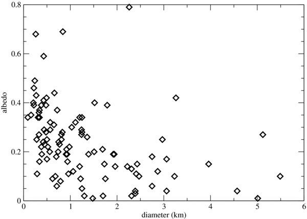
Figure 4. Albedo vs. diameter for our first 101 targets, using fixed-η solutions in all cases. Two objects are off the plot: 42286 (2001 TN41), with modeled pV of 1.03 and diameter 0.7 km, and (433) Eros, with modeled pV of 0.06 and diameter 32 km; see Section 5.3 for discussion of these objects. The approximate errors for each data point may be as large as 25% in diameter and 50% in albedo.
Download figure:
Standard image High-resolution image
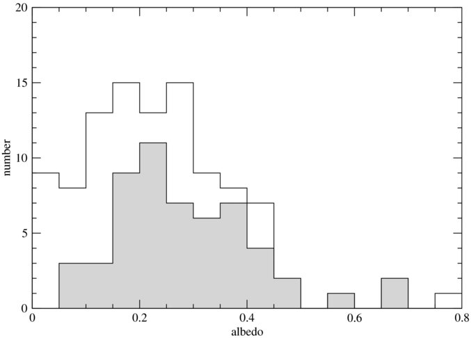
Figure 5. Distribution of albedos for our first 101 targets, using model results derived with the fixed-η model in all cases. The upper line (and clear filled area) is the total for all targets, and counts from the bottom. The lower line (and gray filled area) is the total for the 56 targets smaller than 1 km. The bias against small, dark objects is apparent.
Download figure:
Standard image High-resolution image5.1. Floating η and Fixed η Results
For a subset of our targets we are able to obtain apparently reasonable results by modeling the thermal fluxes at both 3.6 and 4.5 μm. For this purpose we use the full NEATM model (in combination with the optical brightness calculated from H) and derive albedo, diameter, and η, the model parameter that depends on the thermal properties of the body. These "floating-η" fits generally return more accurate results as the properties of each body are solved for individually. However, in the case of our Spitzer data the ratio of the 4.5/3.6 μm thermal flux components varies widely, probably reflecting the significant uncertainty associated with the correction for solar reflected radiation at 3.6 μm (Figure 2). In many cases, NEATM fits fail completely or result in unrealistically high/low albedos and/or η values. We find that setting a filter in the processing pipeline to exclude targets with 4.5/3.6 μm thermal flux ratios outside the range 7–10 gives reasonable floating-η results for all cases passing the filter.
In order to solve for albedo and diameter in the general case (i.e., lacking a reliable 3.6 μm thermal flux value), we assume a value for η based on the object's observational phase angle: η = 0.013α + 0.91, where α is the phase angle in degrees (Wolters et al. 2008). We refer to these solutions as "fixed-η" fits. Since we do not solve for the properties of individual asteroids, these fixed-η solutions are generally less reliable (have larger intrinsic errors) than floating-η fits to two reliable thermal flux values.
Table 2 compares our derived results for the 19 targets passing our thermal flux ratio filter (that is, those objects with realistic floating-η solutions) to their respective fixed-η solutions. The mean fractional difference ((Dfixed − Dfloat)/Dfloat) between the two sets of diameters is −7.5%, a remarkably good agreement, indicating that overall the fixed-η results do not suffer from a serious bias. The mean absolute fractional difference (|(Dfixed − Dfloat)|/Dfloat) is 21%. These comparisons suggest that the additional error introduced by using the fixed-η approach—the only approach possible in most cases—is not large. For the 20% of our targets for which the data warrant a floating-η solution we can gain both an understanding of the surface physical properties of those asteroids and an evaluation of the validity of our fixed-η assumption (M. Mueller et al. 2010, in preparation).
Table 2. Comparison between Floating-η and Fixed-η Model Results
| Target | NEATM Floating-η | Fixed-η | ||||
|---|---|---|---|---|---|---|
| D | pV | η | D | pV | η | |
| (km) | (km) | |||||
| 2100 Ra-Shalom 1978 RA | 2.35 | 0.12 | 1.97 | 2.22 | 0.14 | 1.87 |
| 5604 1992 FEa | 0.61 | 0.38 | 1.56 | 0.71 | 0.28 | 1.86 |
| 67381 2000 OL8 | 0.32 | 0.19 | 1.98 | 0.28 | 0.25 | 1.74 |
| 138937 2001 BK16 | 0.83 | 0.26 | 1.54 | 0.92 | 0.21 | 1.69 |
| 164201 2004 EC | 4.34 | 0.05 | 2.35 | 2.87 | 0.12 | 1.71 |
| 184990 2006 KE89 | 1.59 | 0.18 | 2.06 | 1.24 | 0.29 | 1.64 |
| 1996 EO | 0.39 | 0.27 | 1.63 | 0.42 | 0.24 | 1.73 |
| 1998 SV4 | 0.71 | 0.21 | 1.46 | 0.74 | 0.20 | 1.51 |
| 2002 HF8 | 0.55 | 0.29 | 1.23 | 0.70 | 0.18 | 1.54 |
| 2002 LS32 | 0.82 | 0.14 | 2.33 | 0.57 | 0.29 | 1.67 |
| 2003 SL5 | 0.50 | 0.16 | 2.41 | 0.33 | 0.36 | 1.61 |
| 2003 TL4 | 0.37 | 0.24 | 1.89 | 0.38 | 0.22 | 1.95 |
| 2003 UN12 | 0.98 | 0.08 | 1.24 | 1.25 | 0.05 | 1.49 |
| 2003 WD158 | 0.67 | 0.12 | 2.38 | 0.44 | 0.29 | 1.62 |
| 2004 SB20 | 0.49 | 0.32 | 2.00 | 0.43 | 0.41 | 1.75 |
| 2005 OU2 | 0.26 | 0.63 | 1.22 | 0.34 | 0.37 | 1.68 |
| 2005 UH6 | 0.70 | 0.12 | 2.41 | 0.52 | 0.22 | 1.84 |
| 2006 LF | 0.77 | 0.11 | 2.22 | 0.50 | 0.25 | 1.53 |
| 2006 SY5 | 0.12 | 0.19 | 2.15 | 0.09 | 0.34 | 1.61 |
Notes. The mean fractional difference between the two sets of diameters, ((Dfixed − Dfloat)/Dfloat), is −7.5%; the mean absolute fractional difference, (|(Dfixed − Dfloat)|/Dfloat), is 21%. aWe use H = 17.72 for (5604) 1992 FE (see Section 5.3).
Download table as: ASCIITypeset image
5.2. Results for the Entire Sample
Figure 4 shows derived albedo and diameter for our first 101 targets. We find that around half of our targets have diameters less than 1 km, thus increasing the number of subkilometer NEOs with known properties significantly. These smallest NEOs have a wide range of albedos, from 0.1 to 0.7, implying a wide range of compositions. There are no objects with diameters less than 500 m and albedos less than 0.1 in these initial results. This lack of smallest, darkest NEOs is an observational bias that derives from our sample selection: we observe only those targets that have been reasonably well observed in ground-based (optical) programs, and such programs are biased against small, dark objects.
There are few objects in our sample larger than 1 km that have albedos larger than ∼0.35 (in comparison, many subkilometer objects have albedos this large or larger). This is consistent with the idea that the NEO population continues to be sculpted by collisions (or perhaps disruptive dynamical interactions with planets), in that the smaller objects would be younger, and thus have undergone less space weathering, which darkens surfaces. The darkening timescale at 1 AU is around 1 million years (Strazzulla et al. 2005; Vernazza et al. 2009). Thus, the dichotomy in albedos for large versus small NEOs may indicate that many NEOs smaller than 1 km are quite young.
Figure 5 shows the distribution of albedos for the first 101 targets. We find that the distribution is relatively flat for albedos less than 0.3. The biases here are more complicated than above. Primarily, there is an optical observational bias against dark objects in the smallest size range. However, dark objects may be more common in the larger size range due to space weathering. The overall effect may be that the distribution of albedos in the NEO population shown in Figure 5 may be reasonably representative of NEO composition diversity. Our results here suggest that the NEO population may be approximately equal parts bright (pV ≳ 0.25), moderate (0.1 ≲ pV ≲ 0.25), and dark (pV ≲ 0.1) objects (using somewhat arbitrary cutoffs), implying that a wide range of asteroid taxonomic types may be represented. If borne out, this information would trace key source regions of NEOs in the main belt. However, given the uncertainties in our model results described above, this result is quite preliminary.
Previous work (Morbidelli et al. 2002; Stokes et al. 2003; Stuart & Binzel 2004) predicted that bright S-type asteroids make up 50%–80% of the NEO population, with dark C-type NEOs being the remaining minority. Our distribution of albedos formally is consistent with this prediction, though it might require many of our albedos to be systematically too dark. A systematic error in albedo is indeed likely, due to the systematic errors in H (Section 2.2.3). However, if the catalog H values are systematically too bright then the effect on our albedos would be to make them systematically too bright (i.e., the opposite sense from making our results align with the previous predictions).
There are a number of other results that arise from our first 101 targets; here, we present a preliminary list of forthcoming papers and results. (1) One of these objects, (85938) 1999 DJ4, is a known binary for which we can derive the bulk density (J. Kistler et al. 2010, in preparation). (2) We have observed roughly one dozen of our ground-truth targets, and find that, overall, our results match quite well to those obtained elsewhere (Harris et al. 2010). (3) Within our first 101 targets there are also a number of low delta V targets—that is, targets that spacecraft can approach relatively easily (M. Mueller et al. 2010, in preparation). Diameters for these objects are essential for mission planning, and low albedos can indicate primitive compositions, of interest for various space missions (e.g., Marco Polo, Osiris-REx). (4) We have begun a study of the albedos of objects in our sample with low Tisserand parameter with respect to Jupiter, with the idea of examining whether, as predicted (Levison 1996; Binzel et al. 2004), these objects preferentially derive from the outer solar system (as suggested by low albedos). In our first 101 targets, we have only two targets with TJ < 3 (the nominal cutoff in Levison 1996; Fernandez et al. 2005; DeMeo & Binzel 2008), so our results are presented in Harris et al. (2010). (5) Combining our Spitzer results with results from our ground-based campaign (Section 6) allows us to evaluate the relationship between spectrally determined compositions (through taxonomic typing) and albedo and to measure the uncertainties in the derived albedos for individual objects (C. A. Thomas et al. 2010, in preparation).
5.3. Results for Individual Objects
5.3.1. (433) Eros
A great deal is known about (433) Eros from the NEAR spacecraft mission and supporting ground-based observations. The interpretation of thermal-infrared observations of (433) Eros is complicated by the fact that it can have a very large lightcurve amplitude (up to 1.4 mag) and that its rotation axis lies near the ecliptic plane (λ = 17°, β = 11°; Miller et al. 2002). The mean diameter derived on the basis of the known volume (Cheng 2002) is 17.5 km, whereby previous thermal-infrared measurements have given effective diameters of 14.3 km and 23.6 km at lightcurve minimum and maximum, respectively (Harris & Davies 1999). The disk-averaged albedo of Eros is around 0.22 (Harris & Davies 1999; Li et al. 2004).
The naive fixed-η fit to our Eros data yields an albedo of 0.06 and a diameter of 31.93 km, quite different from the values cited above. A detailed investigation of these data and model results is therefore warranted, both to understand why our model results do not reproduce the expected results, and more broadly to characterize systematic uncertainties present in our modeling.
The line of sight from Spitzer to Eros was around 5° different from Eros' rotation axis at the time of the Warm Spitzer observations. With near pole-on geometry at a phase angle of 365, the effects of rotation/thermal inertia on η are much reduced since the thermal emission is concentrated in the visible hemisphere. Therefore, the adopted relation between η and the phase angle, which embodies a generalized first-order correction for such effects, is not applicable in this unusual case. Harris & Davies (1999) observed Eros at a geometry similar to that of our Spitzer observations (the line of sight to Eros was only 26° away from the rotation axis, at a phase angle of 31°), and found that η = 1.07 gave the best fit. Finally, the appropriate value for H is not 11.16, the mean value employed above in our naive fit, but rather 10.46, which corresponds to lightcurve maximum, appropriate for a pole-on view. Using η = 1.07, H = 10.46, and the Spitzer 4.5 μm (thermal) flux, we find a (maximum) diameter of 22.3 km and pV of 0.23, which are very close to the results of Harris & Davies (1999) and exactly the albedo found by Li et al. (2004).
A remaining outstanding issue is the 3.6 μm flux, which is larger than this model would predict. One solution would be if the reflectance at 3.6 μm is a factor of 2 (or larger) greater than the reflectance at V band; this is significantly different than our standard 40% brighter assumption. Alternatively the G value (slope parameter), which also influences the amount of reflected solar radiation, may be different from the default value of G = 0.15 assumed throughout this work. We have found (J. P. Emery et al. 2010, in preparation) that the 3.6 μm/V reflectance ratio of Eros is about 1.65, higher than 1.4 but not high enough to remove the problem of the excess 3.6 μm flux. However, taking a reflectance ratio of 1.65 we find that we can reproduce the above values of diameter, albedo, and η for Eros by fitting NEATM to both flux measurements with G = 0.34, a value that is much higher than our default value of 0.15, but still within the bounds of reasonable G values, in light of the value G = 0.46 given for Eros by Tedesco (1990, and note that differences in viewing geometry can cause large variations in measured G values).
Further investigation of the influence of assumed G value on floating-η fits to our Warm Spitzer data will be the subject of future work. Since the thermal flux at 4.5 μm is relatively insensitive to the 3.6 μm/V reflectance ratio and G, the uncertainty introduced into the fixed-η results by errors in these parameters is very small. For example, with H = 10.46, G = 0.15, and reflectance ratio of 1.4, the fixed-η diameter result is 30.17 km. Taking H = 10.46, G = 0.34, and reflectance ratio of 1.6, the fixed-η diameter becomes 30.01 km.
The larger conclusion of this analysis is that Eros should act as a reminder of the effects of rotation vectors (as well as cases where G ≠ 0.15) and therefore that the results for individual objects should be treated with caution. However, Eros is also a special case—and especially poorly fit—in some regards. For example, Eros is unusually pole-on in our Spitzer observations. The probability that a randomly oriented rotation pole has an orientation angle less than or equal to θ is L(⩽θ) = (1 − cos θ) (Trilling & Bernstein 2006). Therefore, if NEO rotation axes are distributed isotropically, less than 1% of all NEOs should be observed within 5° of their rotation poles as Eros was. The actual probability is likely even less, since YORP thermal torques will tend to move obliquity values toward 0 or 180° (that is, θ = 90°) (Vokrouhlický et al. 2003; Bottke et al. 2006), and there is some observational evidence of this (La Spina et al. 2004; Kryszczyńska et al. 2007). In other words, it is unlikely that any other of our first 101 targets was observed with this close a pole-on geometry. Therefore, our η/phase angle relationship is likely to be generally appropriate, and many of our other, naive fits are likely to be much more acceptable. The case of (2100) Ra-Shalom is one of these.
5.3.2. (2100) Ra-Shalom
(2100) Ra-Shalom is a well-studied object for which the diameter and albedo have been established as a result of various infrared and radar observing campaigns. It has a lightcurve amplitude of 0.41 mag (Pravec et al. 1998), much lower than that of many other NEOs (compare to Eros, above, with Δmag of 1.4). (2100) Ra-Shalom therefore serves as an excellent test of the viability of our analysis procedures. Shepard et al. (2008) obtained an effective diameter of 2.3 ± 0.2 km and pV of 0.13 ± 0.03 from radar observations. Harris et al. (1998) obtained virtually identical values from thermal-infrared observations. The values obtained for (2100) Ra-Shalom from our warm Spitzer data—(2.35 km, pV of 0.12) and (2.22 km, pV of 0.14) for floating-η and fixed-η, respectively (Table 2)—agree remarkably well with the earlier results (Figure 6). Further work to check the accuracy of our results against other "ground-truth" targets is underway (Harris et al. 2010).

Figure 6. NEATM fit to the Warm Spitzer thermal fluxes for (2100) Ra-Shalom obtained in 2009 August. (The reflected light component has been removed.) This is one of the targets for which the quality of the data enables a floating-η fit to be performed. The resulting diameter and albedo are in good agreement with earlier ground-based results (Delbo' et al. 2003; Shepard et al. 2008). For most of our targets, especially those with high albedos, the uncertainties in the 3.6 μm thermal flux components preclude a floating-η NEATM fit, and we resort to the fixed-η method (Section 4). A comparison of the results obtained with these two methods, and results available in the literature for some of our targets, will facilitate further refinement of the fixed-η method.
Download figure:
Standard image High-resolution image
5.3.3. (5604) 1992 FE
The H value for (5604) 1992 FE provided by Horizons of 16.4 is probably incorrect. Delbo' et al. (2003) used an updated value (H = 17.72) obtained from the lightcurve observations of their co-author Pravec. With this value they obtained an albedo of 0.48. We use H = 17.72 for the results presented in Table 2, where we find a floating-η solution with an albedo of 0.38. This is more reasonable than the very large value (0.69) given in Table 1. This object is known to be a V-type asteroid, so high albedos are expected.
5.3.4. Objects with Unusual Albedos
We derive pV of 1.03 for (42286) 2001 TN41. This albedo is almost certainly too large, as the largest plausible albedo for an NEO is probably not too much larger than 0.5. However, the total uncertainty in albedo for any given object is around a factor of 2; at this level, the true albedo for 2001 TN41 could be 0.5, which would be relatively unsurprising. The CH1/CH2 flux ratio for this object is greater than unity, which is unusual in our sample and can only occur for objects that are cold through being distant or highly reflective (see Figure 2). The large heliocentric distance of 2 AU, the third largest within our sample, confirms that this object is colder than most of our other targets, and its observed fluxes are dominated by reflected sunlight (more than 90% under our assumptions), rendering the calculated thermal fluxes very sensitive to uncertainties in H magnitude. The quantitative characterization of the resulting statistical diameter uncertainty is beyond the scope of this work and will be treated in an upcoming paper (M. Mueller et al. 2010, in preparation). When more accurate H is known, a more accurate albedo can be derived.
The next highest derived albedos are 0.8, 0.68, 0.6, and 0.49 for (4953) 1990 MU, 2001 TX44, (152637) 1997 NC1, and (10302) 1989 ML, respectively. Aside from the first, these albedos are generally plausible. Mueller et al. (2007) found pV of 0.37 for (10302) 1989 ML; our derived value is some 30% higher, no larger than our expected albedo uncertainties.
Four objects in our first 101 targets have derived albedos less than 2%. These values are surprisingly low, and may suffer from errors, especially in H magnitude. However, errors of 50% or more, which would not be surprising at this stage, would raise these albedos to 3% or 4%, values that are consistent with expected values for dark NEOs.
5.3.5. Subkilometer NEOs
Of our first 101 targets, more than half (56) have derived diameters smaller than 1 km. The smallest object observed to date is 2006 SY5, with a derived diameter of 87 m (with a very plausible albedo of 0.34). With expected errors of perhaps 50% on diameter, this object is very likely to be smaller than 150 m, and could be as small as 50 m, depending on the sign of potential errors. These subkilometer bodies are among the smallest NEOs for which physical properties are known. The distribution of albedos for these 56 subkilometer objects is shown in Figure 5. The bias against small objects with low albedos is readily apparent here. Otherwise, these smallest NEOs seem to have the same diverse compositions (as implied by a large range of albedos) that the entire sample has.
6. FUTURE WORK
The ExploreNEOs program has just begun. Some analyses cannot be undertaken until we have most or all of our data in hand. These include a true analysis of the size distribution of NEOs (a large sample size is required for this); thermophysical modeling of certain targets (detailed observations of our ground-truth and multi-visit targets are needed); determining the distribution of albedos in the NEO population, though Figure 5 shows our first results in this direction; and measuring the mean albedo as a function of NEO size (a large sample size is needed for this).
We have also begun a comprehensive ground-based observing program that is a critical component of the larger ExploreNEOs project. Because the H magnitudes of NEOs are typically quite poor, we are carrying out a program of obtaining optical photometry for (ideally) all of the targets in our program. We use a range of telescopes with apertures from 0.36 m to 8 m. We use facilities to which our team has institutional access as well as competed national telescopes and dedicated facilities. As part of this optical photometry program, we will obtain lightcurves for a subset (∼20%) of our targets. We will use this lightcurve data set as a proxy for the lightcurve variability inherent in the larger sample, and thus to understand the errors present in our model results. Both the optical photometry catalog and the lightcurve database will be interesting scientific contributions on their own, of course, and will be presented in forthcoming papers. At the conclusion of the ExploreNEOs program, we will complete a final re-calculation of all model results, incorporating results from this ground-based program. Due to improved H magnitudes, those final errors should be substantially reduced from those presented here.
Our ground-based campaign also includes obtaining spectroscopy and spectrophotometry of several hundred of our targets. The goal of these spectral measurements is to determine taxa and compositions for those targets. We will use these compositional determinations together with our albedo results to understand the compositional distribution within the NEO population. We will measure the correlation between spectrally determined compositions and albedos, and use this relationship to determine by proxy the compositions for those objects in our sample for which we will not obtain spectral information, only albedo.
7. SUMMARY
We have begun a large NEO survey called ExploreNEOs, which uses Warm Spitzer to observe some 700 NEOs at 3.6 and 4.5 μm. We have also begun a comprehensive ground-based observing program that complements the Warm Spitzer data that we will obtain. We have a large number of science goals associated with ExploreNEOs; the overall goal is to explore the history of near-Earth space. We have presented here some fundamental information about the design of our program. We present in this paper results for the first 101 targets in our program. We find that the distribution of albedos in this first sample is quite broad, probably indicating a wide range of compositions within the NEO population. Many objects smaller than 1 km have high albedos (≳0.35), but few objects larger than 1 km have high albedos. This result is consistent with the idea that these objects are collisionally older, and therefore possess surfaces that are more space weathered and therefore darker, or are not subject to other surface rejuvenating events as frequently as smaller NEOs. We find that our nominal results for (2100) Ra-Shalom match previously published values quite closely, while our nominal results for Eros diverge significantly from previous values, though in a readily explainable way. A number of objects have plausible but high (>0.5) albedos. However, given the uncertainties present in our thermal modeling at this time, all of these results are only preliminary. We will continue to refine our thermal models and improve the optical magnitudes for these targets in order to minimize the uncertainties on diameter and albedo. This paper is the first in a series of papers that will present various results from ExploreNEOs.
We acknowledge the thorough and prompt hard work of the staff at the Spitzer Science Center, without whom the execution of this program would not be possible. We thank Michael Mommert (DLR) for help in checking the modeling results given in the data tables. We thank an anonymous referee for making a number of useful suggestions. This work is based in part on observations made with the Spitzer Space Telescope, which is operated by JPL/Caltech under a contract with NASA. Support for this work was provided by NASA through an award issued by JPL/Caltech.
Facility: Spitzer(IRAC) - Spitzer Space Telescope satellite