


ABSTRACT
We have identified 4659 variable objects in the Northern Sky Variability Survey. We have classified each of these objects into one of the five variable star classes: (1) Algol/β Lyr systems including semidetached, and detached eclipsing binaries, (2) W Ursae Majoris overcontact and ellipsoidal variables, (3) long-period variables such as Cepheid and Mira-type objects, (4) RR Lyr pulsating variables, and (5) short-period variables including δ Scuti stars. All the candidates have outside of eclipse magnitudes of ∼10–13. The primary classification tool is the use of Fourier coefficients combined with period information and light-curve properties to make the initial classification. Brief manual inspection was done on all light curves to remove nonperiodic variables that happened to slip through the process and to quantify any errors in the classification pipeline. We list the coordinates, period, Two Micron All Sky Survey colors, total amplitude variation, and any previous classification of the object. 548 objects previously identified as Algols in our previous paper are not included here.
Export citation and abstract BibTeX RIS
1. INTRODUCTION
The Robotic Optical Transient Search Experiment (ROTSE-I; Akerlof et al. 2000) was a project whose main goal was to detect the so-called orphan gamma-ray bursts (GRBs) and provide follow-up for high-energy missions with rapid optical observations. With nearly a year in baseline, observations nearly nightly, and all-sky coverage, the project is an excellent resource for finding variable stars. The data were compiled as the SkyDOT database and released as The Northern Sky Variability Survey (NSVS; Woźniak et al. 2004). The database contains about 14 million unique objects, and we have identified and classified 4659 objects into several variable star classes. This was achieved with period, light curve information, Fourier coefficients, and some manual inspection, to be discussed later.
The identification of pulsating stars is important for the calibration and determination of distance indicators. Early in the 20th century, Cepheids were discovered to have a period–luminosity (and later refined to a period–luminosity–color) relation that makes them useful as distance indicators (see Tammann et al. 2003, 2008 for examples of modern studies). Cepheids typically have periods longer than 1 day and light curves ranging from nearly sinusoidal to strongly asymmetric. Having a larger sample of Cepheids allows for refinement of the relations. However, in old stellar systems, there are no Cepheids for distance estimates, but RR Lyrae variables are present. RR Lyr variables are radial pulsators with periods usually between 0.2 and 1.0 day with light curves similar to Cepheids. RR Lyr variables can also be used as distance indicators as they show a metallicity–luminosity relation (Sandage & Tammann 2006). These stars are essential for use as standard candles in nearby galaxies as well as globular clusters in our own galaxy and also for understanding stellar pulsation and evolution.
The δ Scuti variables are another type of pulsating star in the instability strip. These are typically main-sequence or slightly evolved stars of spectral types of A or F with periods between roughly 0.5 and 7 hr. The δ Scuti stars are divided into two main types: the high amplitude delta Scutis (HADS) and the small amplitude δ Scutis. HADS have photometric variations of more than 0.25 mag while the small amplitude types can have variations on the order of millimagnitudes. The small amplitude class usually pulsates in multiple modes and has nonradial modes, creating a very chaotic light curve as beating occurs. The HADS are typically monotone radial pulsators and have more stable light curves (Laney et al. 2003). As discussed by Breger (2000) and others, mode identification of multimode δ Scuti stars is very difficult, but is very important to constrain stellar pulsation models. Additionally, HADS with stable light curves can be used as a short-period extension of the Cepheid period–luminosity–color relation (Laney et al. 2003).
W Ursae Majoris-type stars (W UMa) are close contact binary systems. They are among the most numerous variable stars in the sky. The stars in W UMa systems are main-sequence stars of spectral types from early A to early K and typically have periods between 0.25 and 1.2 days (Rucinski 2004). Recent theories suggest that W UMa binaries start out as detached systems with P ≈ 2 days and very different masses. The binary loses angular momentum due to magnetized stellar winds and eventually forms a common envelope with mass transfer (Stępień 2006; Eker et al. 2007). Despite having very different mass ratios ranging from q = 0.97 to q = 0.066 (Rucinski et al. 2001), the surface brightness and effective temperature are nearly identical over the entire contact envelope surface. Due to their unique properties, W UMa systems can be used similarly to pulsating stars by using a period–luminosity–color relation as a distance indicator among solar-type stars (Rucinski 2004).
Eclipsing binaries of Algol and β Lyrae type offer a unique opportunity to determine stellar parameters with a high degree of accuracy, including a direct measurement of the radius of each star if the period, inclination, and radial velocity of each star is known. Algol and β Lyrae eclipsing binaries are differentiated by constant variation in the light curve outside of eclipses for the β Lyrae systems to the nearly constant brightness outside of eclipses of the Algol-type systems. Refer to Hoffman et al. (2008) for more information on these eclipsing binaries.
2. ANALYSIS METHOD
The initial requirements for a variable star candidate in the NSVS were the same as those of Hoffman et al. (2008), requiring at least a 0.1 mag variation about the median magnitude and at least 30 observations. This immediately reduced the number of variable star candidates from 14 million in the NSVS to around 100,000 objects.
These candidates are then put through Fourier analysis, magnitude ratio, and phase dispersion minimization routines to determine and identify periodicities in the data. This step is again identical to that of Hoffman et al. However, since we will later be fitting a Fourier series to the data, we invoke an additional constraint on the data of having at least one data point in each 0.05 phase bin. This ensures that the light curve is well sampled at all phases. We compute the median magnitude value in each bin to produce an averaged smoothed light curve. Combined with the magnitude ratio used in Hoffman et al., we determine whether the candidate is a pulsating (one minimum per cycle) or eclipsing/ellipsoidal variable (two minima per cycle). The process involves finding the global minimum and then searching 0.5 in phase from the minimum for a local minimum. If the light curve has another local minimum at this point or is relatively flat (as an Algol with no secondary eclipse might be), it is flagged as an eclipsing/ellipsoidal variable. Otherwise, the candidate is flagged as a pulsating star and the period is halved for the final tabulation. For the Fourier decomposition to follow, candidates flagged as pulsating stars are phased to twice their real period so that all candidates can be directly compared.
The next step in the process is Fourier decomposition (Rucinski 1993). We use the Levenberg–Marquardt nonlinear least-squares fitting routine to fit the following equation (Rucinski 1993) to each light curve:
where θ is the phase and ϕ is the phase offset to compensate for the unknown time of minimum/maximum. While six orders are used for the fit, only the first four are used for classification. If the fit does not converge (i.e., low-order coefficients near zero or unrealistically large values), the routine is run again with slightly different initial conditions. If it fails to converge again, the light curve is phased at integer harmonics of the period. If the fit still does not coverage, the candidate light curve is discarded as this is indicative of a nonperiodic variable or a light curve with insufficient data.
Light curves with periods very close (within 0.001 days) to an integer harmonic of 1 day are discarded. This is usually an indication that the fast Fourier transform performed earlier failed to find significant periodicities in the data. However, there are indeed some real variable objects with such periods that are discarded, but due to the rarity of such objects and the large number of rejected light curves, manual inspection was not performed for these sources.
If a4 has a positive value, the candidate is assigned an initial classification of RR Lyr if the period is less than 1.2 days and as a long-period/Cepheid candidate otherwise. Algol/β Lyrae candidates identified previously in Hoffman et al. (2008) are removed from the candidate list. RR Lyr variables identified in the NSVS by Kinemuchi et al. (2006) are flagged. If a4 is negative, the light curve is analyzed to determine the depths of the primary and secondary minima and combined with period and Two Micron All Sky Survey (2MASS) color information for further classification.
The objects are filtered through the SIMBAD database to find any previous identifications. Since all the objects in the NSVS are relatively bright, almost all of them are expected to have at least been identified by their coordinates (e.g., the Tycho-2 catalog; Høg et al. 2000), though only a small fraction has been previously identified as variables or has been classified.
Objects with |a4| < 0.02 are flagged for close manual inspection. These objects are in the Fourier coefficient region where they could be either RR Lyr or W UMa variables with periods under 1.2 days. The light curves of the 728 objects that met those criteria were manually inspected and classified by their light-curve shape, as the classification by Fourier coefficients is not reliable in this region. However, even after manual inspection, there are likely to be many RR Lyr type variables of subclass RRc misidentified as W UMa variables and vice versa. This is because their light curves can appear nearly identical.
3. RESULTS
The new objects classified as Algol/β Lyr variable are listed in Table 1. This table does not include 548 objects classified as such previously in Hoffman et al. (2008). Table 1 columns include the R.A., decl., NSVS object identification number, period, the J − H, H − K, and K magnitudes extracted from the 2MASS database, the mean ROTSE unfiltered magnitude, the amplitude of oscillations determined from the Fourier fit, any previous identification, any previous classification, and notes. The candidates that have a4 values greater than the line defined by a4 = a2(0.125 − a2) (Rucinski 1997) can be considered β Lyr candidates, as this is the equation defining the envelope for inner contact. Objects that have a4 values less than the line are likely detached eclipsing binaries or Algols. Figure 1 is a plot of the a2 and a4 Fourier coefficients of all 4569 light curves. The curved line is the theoretical limit for inner contact. The detached/semidetached variable star candidates (red crosses) can be considered β Lyr candidates if they are below the curved line. Figure 2 shows some example light curves of objects in this category with two Algol and two β Lyr light curves. The main source of contamination in Table 1 are W UMa type variables. Sometimes the Fourier fit does not reproduce the bottom of the eclipses very well and the algorithm mistakenly identifies the eclipse depths as very different, and thus an Algol system. While all of the objects were manually inspected for obvious period phasing errors, there could possibly be some Algol systems which have little or no secondary eclipse that will be misphased to twice the true period. After manual inspection it was found that of the objects initially identified as Algol/β Lyr candidates, ∼5% were later classified as another class.
Table 1. Algol/β Lyrae Candidates
| R.A. (deg) | Decl. (deg) | Obj ID | Period (days) | J − H | H − K | K | mROTSE | Amp. | ID | Prior Classification | β Lyr? |
|---|---|---|---|---|---|---|---|---|---|---|---|
| 5.12743 | 40.22606 | 3656824 | 0.46286 | 0.218 | 0.025 | 8.427 | 9.988 | 0.474 | V* CN And | W UMa | Yes |
| 5.30759 | 66.08609 | 1617944 | 0.43057 | 0.411 | 0.082 | 10.830 | 12.826 | 0.452 | ... | ... | Yes |
| 6.99914 | 45.62940 | 3661894 | 0.68051 | ... | ... | ... | 13.055 | 0.275 | ... | ... | No |
| 8.15218 | 44.19326 | 3666805 | 7.38015 | 0.537 | 0.163 | 8.735 | 11.432 | 0.362 | ... | ... | No |
| 8.21514 | 49.32876 | 3711864 | 1.74674 | −0.081 | −0.039 | 10.537 | 10.723 | 0.438 | V* V381 Cas | beta Lyr | No |
| 9.50991 | 3.68457 | 11949748 | 4.09002 | 0.563 | 0.152 | 9.298 | 11.999 | 0.434 | ... | ... | No |
| 10.88007 | 62.66553 | 1634344 | 2.20024 | 0.333 | 0.190 | 9.909 | 12.786 | 0.676 | V* BI Cas | Cepheid | No |
| 11.81681 | −19.69551 | 14687578 | 0.48888 | 0.181 | 0.050 | 10.233 | 11.609 | 0.354 | 2MASS J00471603-1941437 | Double Star | Yes |
| 12.40895 | 54.53602 | 1597051 | 0.44594 | 0.223 | 0.054 | 11.946 | 13.311 | 0.209 | ... | ... | Yes |
| 12.43600 | 77.89325 | 307425 | 0.37168 | 0.416 | 0.110 | 10.226 | 12.147 | 0.279 | ... | ... | Yes |
Notes. List of Algol/β Lyrae candidates from the NSVS, not including those identified in Hoffman et al. (2008). "Obj ID" is the NSVS identification number of the object, but other synonym names can exist. The J, H, and K values are taken from the 2MASS database. "mROTSE" is the median magnitude of the object from the NSVS database. "Amp." is the amplitude of variations, computed from the six-order Fourier fit. "ID" is any previous designation from SIMBAD. "Prior Classification" is the SIMBAD classification, if any. The final column is to denote whether the candidate is in the Fourier region where β Lyrae variables are expected to be. "EB" is short for Eclipsing Binary.
Only a portion of this table is shown here to demonstrate its form and content. Machine-readable and Virtual Observatory (VO) versions of the full table are available.
Download table as: Machine-readable (MRT)Virtual Observatory (VOT)Typeset image
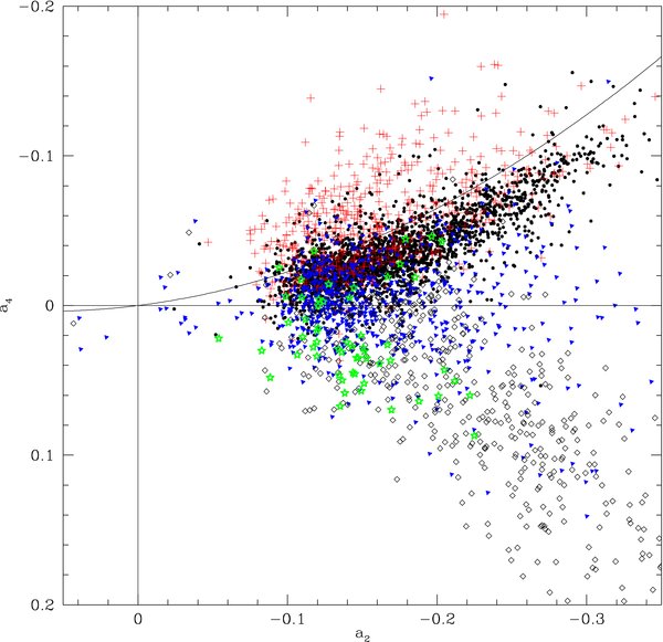
Figure 1. All classified light curves by their Fourier a2 and a4 values. The red crosses are Algol/β Lyr candidates. The curved solid line is the theoretical limit for inner contact, thus the red crosses below the line can be considered β Lyr candidates. The filled black circles are W UMa candidates. The blue triangles are Cepheid/long-period candidates. The open diamonds are RR Lyr candidates, generally having positive a4 values. The green stars are short-period/δ Scuti candidates.
Download figure:
Standard image High-resolution image
Figure 2. Four example light curves of objects from Table 1. The open squares are the Algol NSVS 6750093 (CF Tau), the filled circles are the Algol NSVS 10671817, the open triangles are the β Lyra star NSVS 3801457 (WZ And), and the open circles are the β Lyra star NSVS 6447718.
Download figure:
Standard image High-resolution imageObjects classified as RR Lyr variables are listed in Table 2. These are the open diamonds in Figure 1 and generally have positive a4 values. The vast majority of these objects are of the RRab subclass (asymmetric light curves). The columns of Table 2 are the same as that of Table 1. RR Lyr variables identified by Kinemuchi et al. (2006) are denoted in the last column. Figure 3 shows some example light curves of objects in Table 2. Bumps on the descending branch can sometimes be seen depending on the amplitude and photometric errors. Since there is little overlap in period between the major classes of pulsating stars (δ Scuti, δ Ceph, and RR Lyr), it is fairly easy to classify these objects. There is contamination in the shorter-period candidates, with the most likely contaminant being W UMa stars. There could also be some γ Dor type variables in the sample. As seen in Figure 4, top panel, there is some contamination peaking around 0.35 days, which is due to the W UMa sample (bottom panel). The solid line is the distribution from Samus & Durlevich (2009) and the gray histogram is from the present study. Kinemuchi et al. also had this problem (dotted line). Since W UMa and RRc objects have nearly identical light curves, it is difficult to distinguish them based on single-color photometry alone. Thus, objects in Table 2 with periods less than ∼0.4 days should be treated with suspicion. After manual inspection it was found that of the objects initially identified as RR Lyr candidates, <1% were later classified in another class, though it is clear that there is a significant percentage of the sample that are likely W UMa contaminants. Additionally, ∼56% of our RR Lyr candidates were previously identified by Kinemuchi et al. (2006).
Figure 3. Four example RR Lyr light curves of objects from Table 2. The open squares are NSVS 8184588 (V347 Her), the filled circles are NSVS 13399815, the open triangles are NSVS 16038743, and the open circles are NSVS 13399815 (TV Lib).
Download figure:
Standard image High-resolution image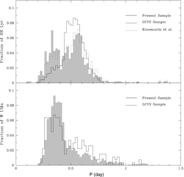
Figure 4. Period distribution of RR Lyr (top) and W UMa (bottom) variable stars in the present sample and in the GCVS. W UMa contamination is evident in the RR Lyr sample due to the secondary peak at 0.35 days. The W UMa distributions are similar. There are 498 RR Lyr candidates in the present sample compared to 4361 in the GCVS, while there are 2332 and 268 W UMa candidates in the present sample and GCVS, respectively
Download figure:
Standard image High-resolution imageTable 2. RR Lyr Candidates
| R.A. (deg) | Decl. (deg) | Obj ID | Period (days) | J − H | H − K | K | mROTSE | Amp. | ID | Prior Classification | Flag |
|---|---|---|---|---|---|---|---|---|---|---|---|
| 4.45233 | 9.88858 | 9088466 | 0.70078 | 0.221 | 0.079 | 10.221 | 12.306 | 0.451 | GSC 00595-00224 | RR Lyr | 1 |
| 5.92965 | 29.40094 | 6302330 | 0.44229 | 0.262 | 0.073 | 8.444 | 9.995 | 0.426 | V* SW And | RR Lyr | 1 |
| 6.99562 | 49.16269 | 3707286 | 0.39201 | 0.165 | 0.062 | 10.878 | 12.376 | 0.357 | ... | ... | 1,2 |
| 8.22575 | 47.14651 | 3713192 | 0.56722 | 0.126 | 0.117 | 11.445 | 13.181 | 0.504 | NSVS 3713192 | RR Lyr | 1 |
| 8.40948 | −15.48750 | 14652041 | 0.57307 | 0.235 | 0.072 | 10.338 | 11.746 | 0.325 | V* RX Cet | RR Lyr | ... |
| 8.80628 | −4.25015 | 11963570 | 0.34447 | 0.126 | 0.021 | 12.186 | 13.425 | 0.401 | ASAS J003514-0415.0 | RR Lyr | 2 |
| 10.18148 | 76.98031 | 258744 | 0.45767 | 0.342 | 0.147 | 11.412 | 13.480 | 0.380 | NSVS 258744 | RR Lyr | 1 |
| 10.27943 | 20.67419 | 9128078 | 0.26860 | 0.104 | 0.081 | 11.217 | 12.357 | 0.274 | ... | ... | 2 |
| 11.98444 | 11.70484 | 9149730 | 0.45559 | 0.261 | 0.042 | 11.094 | 12.336 | 0.549 | ... | ... | 1 |
| 12.39515 | 27.02207 | 6392776 | 0.55464 | 0.243 | 0.033 | 11.749 | 13.385 | 0.557 | V* ZZ And | RR Lyr | 1 |
Notes. List of RR Lyr candidates from the NSVS. The columns are the same as Table 1 except for the last column. "Flag" indicates whether the object was identified by Kinemuchi et al. (2006) or has a period in the region that has a significant probability of being a W UMa candidate. "1" indicates RR Lyr candidate identified by Kinemuchi et al. (2006) and "2" indicates the possible W UMa candidate misidentified as an RR Lyr variable because it has a period in the overlap region (see the text).
Only a portion of this table is shown here to demonstrate its form and content. Machine-readable and Virtual Observatory (VO) versions of the full table are available.
Download table as: Machine-readable (MRT)Virtual Observatory (VOT)Typeset image
Table 3 lists the objects classified as Cepheids and long-period variables. These are denoted as filled blue triangles in Figure 1, and have little correlation in their a2 and a4 values. Due to photometric constraints, it is generally not possible to distinguish between classical and W Vir Cepheids, although it is certainly possible to make such a classification with high-signal/noise photometry and well-sampled light curves. The columns of Table 3 are the same as that of Table 1, except for the final column. The period determined by the Fourier analysis is unreliable when it approaches the baseline of the data. Thus, objects with listed periods of greater than ∼40 days should be treated with suspicion because of the observational window. Figure 5 demonstrates this problem at longer periods. Our sample has significantly more longer-period Cepheids than the GCVS (Samus & Durlevich 2009) would predict. The final column in Table 3 denotes such issues that arise for each object. Figure 6 shows four example light curves of Cepheid candidates from Table 3, and shows the great variety of Cepheid light curves in the database. Unfortunately, it is difficult to distinguish long-period Cepheid and Mira type variables even with 2MASS colors as the color difference is not always statistically significant. Thus, there are some Mira variables that contaminate the Cepheid sample. There is also the possibility of long-period RR Lyr variables in the sample. This possible RR Lyr contamination can be seen by the slight deviation from the GCVS sample near periods of 1 day in Figure 5, though the rest of the period distribution matches quite nicely. As with Vilardell et al. (2007), there is a hint of a secondary peak around 15 days. Less than 1% of these candidates were later classified as another variable star type, but a much higher fraction have questionable periods, as discussed above.
Table 3. Cepheid/Long-Period Variable Candidates
| R.A. (deg) | Decl. (deg) | Obj ID | Period (days) | J − H | H − K | K | mROTSE | Amp. | ID | Prior Classification | Flag |
|---|---|---|---|---|---|---|---|---|---|---|---|
| 4.76052 | 10.67506 | 9089063 | 8.00008 | 0.676 | 0.155 | 10.047 | 13.136 | 0.260 | ... | ... | ... |
| 5.01262 | 63.17977 | 1618500 | 3.80232 | 0.534 | 0.197 | 8.688 | 11.942 | 0.366 | V* CT Cas | Classical Cepheid | ... |
| 5.48246 | 76.45018 | 206147 | 153.84758 | 0.917 | 0.294 | 6.552 | 11.393 | 1.055 | V* AP Cep | Mira | 1,4 |
| 6.40826 | 64.23016 | 1621453 | 3.02118 | 0.567 | 0.215 | 8.622 | 11.816 | 0.384 | V* AS Cas | Cepheid | ... |
| 7.58256 | 41.17675 | 3666194 | 37.03739 | 0.659 | 0.146 | 7.801 | 10.814 | 0.343 | ... | ... | ... |
| 8.05838 | 79.24916 | 254790 | 43.47868 | 0.541 | 0.179 | 10.147 | 12.901 | 0.233 | ... | ... | ... |
| 9.13736 | 43.09769 | 3670906 | 24.39048 | 0.614 | 0.170 | 8.444 | 11.392 | 0.299 | ... | ... | ... |
| 9.18560 | 62.27422 | 1630019 | 6.21124 | 0.638 | 0.317 | 8.350 | 11.971 | 0.302 | V* FW Cas | Classical Cepheid | ... |
| 9.32766 | 63.21600 | 1629613 | 3.19492 | 0.447 | 0.225 | 7.784 | 10.975 | 0.271 | V* V827 Cas | Classical Cepheid | ... |
| 9.61944 | 74.88698 | 212948 | 52.63208 | 0.828 | 0.286 | 8.200 | 12.083 | 0.492 | ... | ... | ... |
Notes. List of Cepheid/long-period variable candidates from the NSVS. The columns are the same as Table 1 except for the last column. "Flag" denotes one of the three flags on the object. "1" indicates the possible false period, as discussed in the text; "2" indicates that the candidate exhibits irregular photometric variations; "3" indicates that the candidate exhibits semiregular photometric variations; "4" indicates that the candidate does not contain sufficient data for classification, but is variable.
Only a portion of this table is shown here to demonstrate its form and content. Machine-readable and Virtual Observatory (VO) versions of the full table are available.
Download table as: Machine-readable (MRT)Virtual Observatory (VOT)Typeset image

Figure 5. Period distribution of Cepheids in the present sample and in the GCVS. The large difference between the two at periods greater than approximately 40 days is due to bias in our observational window function, as discussed in the text. The small difference near 1 day is evidence of some RR Lyr contamination, though the rest of the distribution matches nicely.
Download figure:
Standard image High-resolution image
Figure 6. Four example Cepheid light curves of objects from Table 3. The open squares are NSVS 9945092 (V347 Her), the filled circles are NSVS 1480188 (DT Cas), the open triangles are NSVS 2023703, and the open circles are NSVS 1225362.
Download figure:
Standard image High-resolution imageObjects classified as W UMa type variables are listed in Table 4. This is the most common classification of the variables, which is expected since ∼95% of all variable stars in the solar neighborhood are W UMa type (Eggen 1967). The W UMa candidates are denoted as filled black circles in Figure 1 and generally fall below the curved line of theoretical inner contact. Figure 7 shows some example W UMa light curves for objects listed in Table 4. The most likely contaminant is RR Lyr variables of the RRc subtype. Without color information and higher precision photometry, W UMa and RRc variables cannot be easily differentiated. There can also be some β Lyr objects in this table if the Fourier fit failed to reproduce the eclipse depths accurately. There can also be ellipsoidal variables such as RS CVn stars in the table that are difficult to distinguish with the present data set. The bottom panel of Figure 4 shows a comparison of the period distribution between the NSVS sample and the W UMa objects in the GCVS (Samus & Durlevich 2009). The distributions match quite well considering our sample consisted of almost nine times more candidates than listed in the GCVS. The slight oversampling at the peak is likely due to RRc contamination. Approximately 5% of these W UMa candidates were later reclassified as Algol/β Lyr candidates. An unknown, but relatively significant fraction is likely RRc variables.
Table 4. W UMa Candidates
| R.A. (deg) | Decl. (deg) | Obj ID | Period (days) | J − H | H − K | K | mROTSE | Amp. | ID | Prior Classification |
|---|---|---|---|---|---|---|---|---|---|---|
| 4.04480 | 27.57268 | 6296844 | 0.32537 | 0.391 | 0.070 | 12.021 | 13.015 | 0.334 | ... | ... |
| 4.05871 | 22.16697 | 6297555 | 0.42079 | 0.247 | 0.042 | 10.081 | 11.670 | 0.275 | 2MASS J00161408+2209583 | Double Star |
| 4.24034 | 18.02906 | 9108070 | 0.55326 | 0.155 | 0.034 | 11.632 | 12.749 | 0.273 | ... | ... |
| 4.25655 | 16.99402 | 9108161 | 0.37701 | 0.296 | 0.068 | 11.760 | 13.132 | 0.490 | ... | ... |
| 4.52041 | 45.82038 | 3652820 | 0.42097 | 0.262 | 0.051 | 10.988 | 12.298 | 0.425 | [GGM2006] 3698633 | Double Star |
| 4.80301 | 33.01988 | 6330220 | 0.51008 | 0.177 | 0.059 | 11.461 | 12.843 | 0.286 | ... | ... |
| 4.86766 | 46.98171 | 3699648 | 0.33273 | 0.430 | 0.101 | 10.413 | 12.293 | 0.346 | 2MASS J00192761+4658476 | Double Star |
| 5.14669 | 40.07088 | 3656944 | 0.29705 | 0.399 | 0.142 | 9.868 | 12.070 | 0.281 | ... | ... |
| 5.22280 | 12.10681 | 9089969 | 0.38738 | 0.259 | 0.083 | 11.280 | 13.054 | 0.538 | ... | ... |
| 5.26916 | 32.48753 | 6332027 | 0.34898 | 0.310 | 0.092 | 11.476 | 13.088 | 0.278 | ... | ... |
Notes. List of W UMa candidates from the NSVS. The columns are the same as Table 1 without the last column.
Only a portion of this table is shown here to demonstrate its form and content. Machine-readable and Virtual Observatory (VO) versions of the full table are available.
Download table as: Machine-readable (MRT)Virtual Observatory (VOT)Typeset image

Figure 7. Four example W UMa-type light curves of objects from Table 4. The open squares are NSVS 7330183, the filled circles are NSVS 9172090, the open triangles are NSVS 14347517 (MU Aqr), and the open circles are NSVS 182245 (WZ Cep).
Download figure:
Standard image High-resolution imageThe final table is Table 5, which lists the short-period variables. These are objects with periods less than 0.2 days and are denoted as green stars in Figure 1. The objects in this list are likely dominated by δ Scuti variables, though there could be a few β Ceph variables (pulsating early B-type giants/subgiants) in the list. The δ Scuti stars in this list are necessarily monoperiodic as any significant beating of modes would have blurred the light curve over the long time period of the NSVS and thus would have been rejected by our selection criteria. Figure 8 shows example NSVS δ Scuti light curves. Multiperiodic pulsating stars could be detected by multiple Fourier transform iterations, but because of the low-amplitude nature of these objects and the relatively poor photometric precision of the NSVS data, this was not attempted. Less than 1% of the candidates were later reclassified after manual inspection.
Table 5. Short-Period/δ Scuti Candidates
| R.A. (deg) | Decl. (deg) | Obj ID | Period (days) | J − H | H − K | K | mROTSE | Amp. | ID | Prior Classification |
|---|---|---|---|---|---|---|---|---|---|---|
| 13.82631 | 23.16337 | 6396433 | 0.07869 | 0.053 | 0.025 | 9.993 | 10.987 | 0.343 | V* GP And | delta Scuti |
| 16.44664 | 44.58441 | 3766041 | 0.09449 | 0.140 | 0.055 | 11.391 | 12.663 | 0.330 | - | - |
| 17.60260 | 27.32238 | 6407330 | 0.08698 | 0.092 | 0.047 | 11.740 | 12.925 | 0.275 | - | - |
| 22.46037 | 9.75614 | 9215759 | 0.19324 | 0.279 | 0.041 | 11.584 | 13.133 | 0.180 | ... | ... |
| 26.11626 | 37.98158 | 3844113 | 0.10694 | 0.065 | 0.042 | 12.013 | 13.298 | 0.406 | ... | ... |
| 29.47881 | −18.96304 | 14742359 | 0.06478 | 0.098 | 0.067 | 12.075 | 13.220 | 0.339 | - | - |
| 50.67778 | 39.10968 | 4156098 | 0.11009 | 0.174 | 0.080 | 11.177 | 12.476 | 0.274 | ... | ... |
| 56.83144 | 63.37801 | 2046352 | 0.03910 | 0.170 | 0.039 | 11.987 | 13.322 | 0.247 | V* BL Cam | Pulsating Star |
| 74.33535 | 79.34848 | 448314 | 0.14031 | 0.121 | 0.073 | 10.774 | 12.062 | 0.329 | ... | ... |
| 89.83542 | 20.03451 | 9627247 | 0.20125 | 0.185 | 0.067 | 9.811 | 11.401 | 0.285 | V* V337 Ori | Variable Star |
Notes. List of short-period/δ Scuti candidates from the NSVS. The columns are the same as Table 1 without the last column.
Only a portion of this table is shown here to demonstrate its form and content. Machine-readable and Virtual Observatory (VO) versions of the full table are available.
Download table as: Machine-readable (MRT)Virtual Observatory (VOT)Typeset image

Figure 8. Four example short-period variable light curves from Table 5. These are most likely δ Scuti variables. The open squares are NSVS 3766041, the filled circles are NSVS 14542347 (CY Aqr), the open triangles are NSVS 7856175 (AW CrB), and the open circles are NSVS 5164768 (YZ Boo).
Download figure:
Standard image High-resolution imageDuring the manual inspection process, some light curves were noted as unusual in their characteristics. Figures 9–12 are examples of such objects. Figure 9 is EQ CMa, previously identified as an Algol binary. The light curve is quite unusual for an Algol system, with unequal light at phases 0.25 and 0.75. This could be due to a spotted surface, or that the system is actually a cataclysmic variable (CV) and we are seeing the hotspot being eclipsed. NSVS 5455133, whose light curve is plotted in Figure 10, was previously identified as an eclipsing binary in SIMBAD. The light curve shows a well-defined primary eclipse, but the secondary eclipse, which appears to have nearly the same depth as the primary is very poorly defined. Phasing errors are unlikely as the cause because only the secondary is not well defined and the data are spread over many months. A variable spotted surface on the secondary star could be the cause. Figure 11 shows another unusual light curve, NSVS 4491084, an object with no prior identification. There is a hint of a secondary eclipse at phase 0.5. Like EQ CMa, this could be a spotted system or a CV, though the odd saw-tooth shaped light curve outside of eclipse is unusual. Finally, Figure 12 shows a previously unclassified object, NSVS 4027822, with unequal light at phases 0.25 and 0.75. This is most likely a heavily spotted W UMa or spotted ellipsoidal RS CVn system because of the equal minima. All these systems require follow-up observations to determine their true nature.

Figure 9. Unusual light curve of NSVS 15225915 (EQ CMa). The object is listed as an Algol in the literature.
Download figure:
Standard image High-resolution image
Figure 10. Unusual light curve of NSVS 5455133. The primary eclipse is well defined, while the secondary is not, despite appearing to have the same depth. The data were gathered over many nights, thus the variations are intrinsic to the object.
Download figure:
Standard image High-resolution image
Figure 11. Unusual light curve of NSVS 4491084. Our pipeline classified the object as a Cepheid due to the saw-tooth light curve and 5.34 day period, but the apparent eclipse is most unusual. The object could be a CV, a spotted system, or the very unlikely case of an eclipsing system with the same period as the pulsating component.
Download figure:
Standard image High-resolution image
Figure 12. Unusual light curve of NSVS 4027822. With a period of 0.387 days, the object is most likely a spotted W UMa system, but such a strong effect due to the spots would be unusual.
Download figure:
Standard image High-resolution imageSome objects with unusual light curves can be classified incorrectly with the techniques we have used. An example of such an object that was rejected after manual inspection is NSVS 6300521 (RX J0019.8+2156, QR And). Figure 13 shows the NSVS light curve of the object. Our routine classified the asymmetrical saw-toothed light curve as an RR Lyr star due to the ∼15 hr period of the object, but the object is actually a supersoft X-ray binary system with an unusual light curve. While such a situation is rare, there will be objects in our tables whose true nature is nothing like the variable class that we have assigned.
Figure 13. Light curve of NSVS 6300521 (RX J0019.8+2156, QR And). Our method classified this object as an RR Lyr due to the period and light-curve shape, yet the object is actually an X-ray binary. This is an example of how unusual light-curve characteristics can lead to an incorrect classification.
Download figure:
Standard image High-resolution image
4. SUMMARY
Using a combination of Fourier coefficients, light-curve properties, period, and color information, 4659 variable objects in the NSVS were identified and classified into one of the five categories. The method greatly improves upon Hoffman et al. (2008) as evidenced by nearly twice as many Algol/β Lyr candidates found by this method. The main improvement is the fact that Fourier decomposition allows for light curves with only partial coverage of an eclipse to be useful. The method also almost doubled the number of identified RR Lyr variables in the NSVS database as found by Kinemuchi et al. (2006). If the classification of the W UMa and Cepheid variables are confirmed, they will also greatly increase the number of such objects known. With these variable stars, we have now exhausted the variable objects in the NSVS using our techniques. While more could potentially be found by relaxing the initial selection criteria, the large increase of false-positives would mean that more manual inspection would be required. A more productive use of the method is to apply it to other all-sky survey projects currently coming online (e.g., Pan-STARRS, LSST, etc.). The higher precision photometry and multicolor data of such surveys make them ideal for our pipeline to be applied as the misidentifications and false-positives would be reduced dramatically over that of the NSVS.
The total misidentification rate, where a candidate was later moved to another variable star class after manual inspection, is ∼4%. However, the true failure rate is higher, mainly due to the W UMa/RRc degeneracy problem, errors in the manual inspection, and the quality of the data. Approximately 15% of the total candidates were discarded after manual inspection due to poor data quality, or the obvious nonperiodicity of the data resulting from Fourier fitting errors. We expect that this fraction can be dramatically reduced by further refinement of the Fourier peak selection criteria outlined in Hoffman et al. (2008). Lower photometric errors would also reduce the discarded and misidentification rates, and lower-amplitude multimode systems could be identified.
This publication makes use of the data from the Northern Sky Variability Survey created jointly by the Los Alamos National Laboratory and University of Michigan. The NSVS was funded by the Department of Energy, the National Aeronautics and Space Administration, and the National Science Foundation.