


ABSTRACT
Observations of the 2007 March 18 occultation of the star P445.3 (2UCAC 25823784; R = 15.3) by Pluto were obtained at high time resolution at five sites across the western United States and reduced to produce light curves for each station using standard aperture photometry. Global models of Pluto's upper atmosphere are fitted simultaneously to all resulting light curves. The results of these model fits indicate that the structure of Pluto's upper atmosphere is essentially unchanged since the previous occultation observed in 2006, leading to a well-constrained measurement of the atmospheric half-light radius at 1291 ± 5 km. These results also confirm that the significant increase in atmospheric pressure detected between 1988 and 2002 has ceased. Inversion of the Multiple Mirror Telescope Observatory light curves with unprecedented signal-to-noise ratios reveals significant oscillations in the number density, pressure, and temperature profiles of Pluto's atmosphere. Detailed analysis of this highest resolution light curve indicates that these variations in Pluto's upper atmospheric structure exhibit a previously unseen oscillatory structure with strong correlations of features among locations separated by almost 1200 km in Pluto's atmosphere. Thus, we conclude that these variations are caused by some form of large-scale atmospheric waves. Interpreting these oscillations as Rossby (planetary) waves allows us to establish an upper limit of less than 3 m s−1 for horizontal wind speeds in the sampled region (radius 1340–1460 km) of Pluto's upper atmosphere.
Export citation and abstract BibTeX RIS
1. INTRODUCTION
Acting quite differently from the quiescent body of gas that might be expected for an atmosphere so far from the Sun's energy source, Pluto's atmosphere has been measured in recent years to have increased in pressure by at least a factor of two (Elliot et al. 2003b; Sicardy et al. 2003) since its discovery in 1988. This large-scale change has been observed using the technique of stellar occultation (Elliot & Olkin 1996), monitoring a star's light as it passes through the atmosphere when Pluto moves in front of that star. Previous occultation observations in 1988 (Millis et al. 1993), 2002 (Elliot et al. 2003b; Sicardy et al. 2003), and 2006 (Elliot et al. 2007) established the overall size and structure of Pluto's atmosphere, including the dramatic increase in pressure between 1988 and 2002 and the possibility of thermal gradients (Elliot et al. 1989; Eshleman 1989; Hubbard et al. 1990) or haze (Elliot & Young 1992; Elliot et al. 2003b), resulting in abrupt changes in light-curve slopes. However, while these previous observations provided significant hints about large-scale variations in Pluto's overall atmospheric structure, they were not of sufficient signal-to-noise ratio (S/N) to fully analyze smaller-scale features apparent in the data (Elliot et al. 2003a; Pasachoff et al. 2005).
This paper presents optical data for the 2007 March 18 observations of Pluto's atmosphere obtained via stellar occultation, as well as a detailed analysis of oscillations seen in the upper atmosphere, with a possible model for the genesis of these effects based on Rossby waves. This model, if an accurate description of the present wave structures, allows the calculation of upper and lower limits on high-altitude wind speeds in Pluto's upper atmosphere.
2. OBSERVATIONS
Observations of the 2007 March 18 occultation of the star P445.3 (McDonald & Elliot 2000) by Pluto were made by our collaboration at five sites across the western United States, and from other sites by other groups (see Figure 1 for a map of our observation sites). We successfully obtained data at each of the following sites: the Multiple Mirror Telescope Observatory (MMTO; 6.5 m), Large Binocular Telescope Observatory (LBTO; 8.4 m), Magdalena Ridge Observatory (MRO; 2.4 m), US Naval Observatory, Flagstaff Station (USNO; 1.55 m), and Fremont Peak Observatory (FPO; 0.32 m). Observations using our consortium's Portable Occultation, Eclipse, and Transit Systems (POETS; Souza et al. 2006; Gulbis et al. 2008) were attempted at MMTO, LBTO, MRO, and USNO for high-speed image cadence with GPS-calibrated timing. Unfortunately, telescope-commissioning issues prevented mounting POETS at LBTO, and resulted in our using the facility guide camera at that station. These LBTO observations were recorded using a Sloan r' filter having a central wavelength of 6400 Å.

Figure 1. Map of occultation stations in the western United States: stations plotted are (from south to north) the MMTO (6.5 m), LBTO (8.4 m), MRO (2.4 m), USNO (1.55 m), and FPO (0.32 m). The blue line and its error bars show an estimate (Elliot et al. 2007) of Pluto's surface radius (for scale only, surface effects are not seen in the light-curve data.) The half-light radius (1207 ± 4 km) is given by the dashed line and represents the southern limit of the region from which the stellar flux would have been seen to drop by at least half. The dotted lines farther south depict the extent of the atmosphere, with the southernmost line placed where the stellar flux would have been seen to drop by only 2%. Note that the event's center line is well off the northern limit of the map; hence, all light curves obtained are in the same Pluto hemisphere. (Map by Sharron Macklin, Williams College Office of Information Technology.)
Download figure:
Standard image High-resolution imageAll POETS observations were unfiltered. This technique resulted in the effective passband of the observations being determined by the spectral response of the CCD camera combined with the stellar spectrum from P445.3. We estimate the wavelength of our maximum sensitivity for the POETS observations to be about 7400 ± 500 Å. All POETS observations for this event were taken in the conventional (non-electron-multiplying) 1 MHz mode with a read noise less than 6e− pixel−1 (Souza et al. 2006; Gulbis et al. 2008).
The observations at MMTO were carried out simultaneously in visible and infrared (IR) wavelengths by co-mounting POETS with the PISCES wide-field IR camera (McCarthy et al. 2001) and splitting the signal with a dichroic beamsplitter at approximately 1 μm. The PISCES IR data have an effective wavelength of 16500 Å and are discussed by McCarthy et al. (2008).
Observations at FPO were carried out using a Bessel I filter with an SBIG ST-10XME camera. We estimate an effective wavelength of 7900 Å for this configuration.
The detailed parameters of all observations are summarized in Tables 1 and 2.
Table 1. Observational Sitesa
| Site | Telescope (m) | East Longitude (ddd mm ss) | Latitude (dd mm ss) | Altitude (km) | Observers |
|---|---|---|---|---|---|
| MMTO | 6.5 | −110 53 04 | 31 41 19 | 2.61 | Benecchi, Kulesa, McCarthy, Person |
| LBTO | 8.4 | −109 53 31 | 32 42 04 | 3.19 | Babcock, Hill |
| USNO | 1.55 | −111 44 23 | 35 11 02 | 2.31 | Levine |
| MRO | 2.4 | −107 11 05 | 33 58 36 | 3.18 | McKay, E. Ryan, W. Ryan, Souza |
| FPO | 0.32 | −121 29 55 | 36 45 37 | 0.84 | Meyer, Wolf |
Note. aOrdered by data quality (see Table 2).
Download table as: ASCIITypeset image
Table 2. Instrumental Parameters
| Site | Instrument | Effective Wavelengtha (Å) | Cadence (Hz) | S/Nb |
|---|---|---|---|---|
| MMTO | PISCES | 16500 (H filter) | ∼2 | 490 |
| MMTO | POETS | 7400 ± 500 (unfiltered) | 4 | 336 |
| LBTO | Guide Camera | 6400 (r' filter) | ∼0.20 | 88 |
| USNO | POETS | 7400 ± 500 (unfiltered) | 2 | 70 |
| MRO | POETS | 7400 ± 500 (unfiltered) | 2 | 45 |
| FPO | SBIG ST-10XME | 7900 (I filter) | 0.25 | 8 |
Notes. aThe MMTO utilized a dichroic beamsplitter which split the light at about 1 μm for simultaneous visible and IR observations. bThe S/N in the time that the shadow moves a distance of 60 km (approximately one pressure scale height). This was calculated from a portion of the light curves outside the occultation. The MMTO S/N value is higher for the IR curve than for the visible as the background noise contributed by Pluto–Charon was lower in the IR.
Download table as: ASCIITypeset image
3. LIGHT-CURVE GENERATION
All light curves were generated from the data with frame-by-frame synthetic aperture photometry to extract the combined signal of Pluto, Charon, and the occultation star in a single aperture. This procedure was repeated for a nonvarying calibration star in the frame of observation to account for variable atmospheric transmission. Varying synthetic aperture sizes were used, with the optimal aperture being chosen by maximizing the S/N of the unocculted (and therefore unvarying) signal. The calibrated light curves (Pluto, Charon, and P445.3 signals summed and then divided by the comparison star) were then compared to the raw uncalibrated light curves. If visible differences were noted, the calibrated light curve was used. If the two curves appeared to have the same shape upon visual inspection, indicating stable atmospheric transmission for the duration of the occultation, the raw uncalibrated light curve was used. This was done because the calibration process added noise to the occultation signal since the light from Pluto, Charon, and P445.3 combined was significantly brighter than that from nearby comparison stars. This analysis resulted in raw light curves being used from the MMTO and USNO stations while calibrated light curves were used from the other stations.
Two of the light curves exhibit gaps in the locations of unusable data resulting from problems with weather (variable cloud cover at MRO) and equipment (tracking difficulties with LBTO). However, given the precise timing available from our GPS systems and the known locations of the telescopes, even partial curves can be easily included in the global analysis (see the next section.) The five resulting light curves, as used, are displayed in Figure 2.

Figure 2. Plot of all visible light curves: the usable portions of all visible light curves obtained (ordered by decreasing S/N) are plotted here. Each curve runs from 0 to 1 in normalized stellar signal from P445.3. Note that those curves to the south (such as MMTO) did not penetrate deeply enough to be brought down to the half-light level, while the northernmost curve (FPO) was deeper in the shadow. The gaps in the data are due to either atmospheric effects (clouds and fog) or telescope anomalies (tracking failures) that resulted in no useful data being obtained where not plotted. All plotted data were included in the fitting. Since the timing of even incomplete curves was precise (using GPS), and the telescope locations are well known, partial curves can be included in the fits, subject to weighting by the square of their S/N.
Download figure:
Standard image High-resolution image4. LIGHT-CURVE MODEL FITTING
We fit the light-curve data to an atmospheric model based on that described by Elliot & Young (1992). The model postulates a thermal structure of the form [T(r) = Th(r/rh)b], where T(r) is the temperature as a function of r (radius), rh is the half-light radius, Th is the temperature at half light, and b is a parameter describing the thermal gradient. For b = 0, the atmosphere is isothermal. The basic assumption of our model is that the overall radial structure of Pluto's upper atmosphere is the same all around the body, the same assumption used by Elliot et al. (2007). Since there was no evidence of an occultation by the limb of the body, and the initial astrometric solutions indicated one was not to be expected, the lower boundary was set to a value such that no surface effects entered into the final model light curves. A one-limb model was used. A small percentage of the light would have been contributed by refraction around the far limb, but as our light curves were all far from central, this effect can be safely neglected. The data points of each light curve were registered with GPS timing and their individual telescope coordinates (as given in Table 1) in order to place all light curves in a consistent reference system for fitting. The final coordinates of each point were subtracted from the JPL PLU013 ephemeris for Pluto (Chamberlin 2005) to provide a fixed Pluto-centric reference plane. All five light curves were then fitted simultaneously, resulting in both final occultation geometry and atmospheric parameters following the technique of Elliot et al. (2007).
The parameters of the model fit are given in column 1 of Table 3. The global atmospheric parameters that applied to all light curves are (1) the half-light radius (rh); (2) the gravitational-to-thermal energy ratio, lambda (λ); and (3) the thermal gradient index (b). See Elliot & Young (1992) for a precise definition of these quantities. The global astrometric parameters are the shadow-center offsets in right ascension (R.A.) and declination (decl.), f0 and g0, as defined by Elliot et al. (1993). These offsets represent a combination of the errors in star position and offsets in Pluto's position from its ephemeris. Specific parameters that apply to each station individually are (1) the full-scale signal (when the star was not occulted), (2) the slope of the full-scale signal, and (3) the offset of the "background fraction" from its nominal value. We call the background fraction the portion of the full-scale signal that was not attributable to the star (i.e., Pluto, Charon, moonlight, and anything else).
Table 3. Model Fits to Light Curves
| Parameter | Fit #1 | Fit #2 | Fit #3 | Fit #4 |
|---|---|---|---|---|
| Half-light radius, rh (km) | 1281.7 ± 4.6 | 1295.8 ± 4.6 | 1291.1 ± 4.6 | 1276.1 |
| Lambda (isothermal equivalent) | 18.3 | 18.3 | 18.3 | 17.9 ± 1.1 |
| Thermal gradient power index, b | −2.2 | −2.2 | −2.2 | −1.9 ± 0.8 |
| Offset in R.A., f0 (km) | −3034.7 ± 1.8 | −3040.6 ± 1.8 | −3038.6 ± 1.8 | −3037.3 ± 2.1 |
| Offset in decl., g0 (km) | −808.9 ± 4.7 | −788.5 ± 4.7 | −795.1 ± 4.7 | −797.2 ± 4.1 |
| MMTO IR, number of points | 2100 | 2100 | 2100 | 2100 |
| Background fraction offseta | 0.010 ± 0.002 | 0.0 | 0.0 | 0.0 |
| Slope | 0.17 ± 0.01 | 0.17 ± 0.01 | 0.17 ± 0.01 | 0.17 ± 0.01 |
| Full scale | 10,029 ± 3 | 10,035 ± 3 | 10,026 ± 3 | 10,026 ± 3 |
| MMTO Vis, number of points | 3000 | 3000 | 3000 | 3000 |
| Background fraction offseta | 0.0 | −0.030 ± 0.002 | 0.0 | 0.0 |
| Slope | 0.25 ± 0.02 | 0.25 ± 0.02 | 0.25 ± 0.02 | 0.25 ± 0.02 |
| Full scale | 9944 ± 6 | 9947 ± 6 | 9927 ± 5 | 9930 ± 6 |
| FPO, number of points | 401 | 401 | 401 | 401 |
| Background fraction offseta | −0.04 ± 0.25 | −0.05 ± 0.25 | −0.05 ± 0.25 | −0.05 ± 0.25 |
| Slope | −0.13 ± 0.13 | −0.13 ± 0.13 | −0.13 ± 0.13 | −0.13 ± 0.13 |
| Full scale | 9609 ± 153 | 9609 ± 153 | 9609 ± 154 | 9609 ± 154 |
| LBTO, number of points | 232 | 232 | 232 | 232 |
| Background fraction offseta | 0.03 ± 0.01 | 0.03 ± 0.01 | 0.03 ± 0.01 | 0.03 ± 0.01 |
| Slope | 0.04 ± 0.04 | 0.04 ± 0.04 | 0.04 ± 0.04 | 0.04 ± 0.04 |
| Full scale | 10,017 ± 17 | 10,017 ± 17 | 10,017 ± 17 | 10,017 ± 17 |
| MRO, number of points | 797 | 797 | 797 | 797 |
| Background fraction offseta | 0.03 ± 0.02 | 0.02 ± 0.02 | 0.02 ± 0.02 | 0.02 ± 0.02 |
| Slope | −1.07 ± 0.76 | −1.11 ± 0.76 | −1.10 ± 0.76 | −1.10 ± 0.76 |
| Full scale | 9718 ± 203 | 9707 ± 202 | 9709 ± 203 | 9710 ± 203 |
| USNO, number of points | 1209 | 1209 | 1209 | 1209 |
| Background fraction offseta | 0.00 ± 0.01 | 0.01 ± 0.01 | 0.01 ±0.01 | 0.01 ±0.01 |
| Slope | 1.07 ± 0.11 | 1.07 ± 0.11 | 1.07 ± 0.11 | 1.07 ± 0.11 |
| Full scale | 10,226 ± 30 | 10,227 ± 30 | 10,227 ± 30 | 10,227 ± 30 |
| Reduced chi square | 1.033 | 1.029 | 1.041 | 1.044 |
Note. Bold indicates our adopted solution. aIn units of normalized stellar signal.
Download table as: ASCIITypeset image
Sections covering a 360 s interval surrounding the occultation portion of each light curve were selected for fitting. To facilitate the weighting of the data points, each curve was (approximately) normalized between 0 (star fully occulted) and 10,000 (star fully visible). Weights used in the fitting were calculated from the variance of the pre-occultation signal. The background fractions used to generate the normalized curves for the MMTO data were 0.631 ± 0.007 for the visible POETS data and 0.167 ± 0.002 for the IR PISCES data. The difference between these two numbers results from the star being much brighter in the IR than in the visible when compared with Pluto. The normalized curves were determined from separated photometry taken earlier and later in the night while Pluto-Charon and P445.3 were well resolved. The background fractions for the other stations were allowed to be free in the fitting as the S/N of these data sets did not allow photometry as accurate as that obtained at the MMTO. Table 3 gives the results of these calibrations based upon the fits.
Although many fits were carried out, we present just four in Table 3. All of the data in these fits were weighted inversely as the (S/N)2 (see Table 2) of their individual stations. Since all light curves were south of the planet's center, the fits did not have significant sampling all the way around the limb for simultaneously fitting the shadow radius (rh) and atmospheric parameters (λ, b), resulting in greater uncertainties in these values. To stabilize the fits, the lambda and thermal gradient parameters were fixed to the values (λ = 18.3, b = −2.2) determined by Elliot et al. (2007) during the 2006 occultation. As MMTO was the station with the highest S/N, Fit #1 fixes the MMTO visible light-curve background fraction offset at 0 and allows other stations to adjust to it. Fixing the background fraction offset to 0 for a station is equivalent to assuming that the calculated photometric background fraction for that station is correct. Fit #2 fixes the MMTO IR curve background fraction offset to 0. Fit #3 fixes the background fractions for both of the MMTO curves. Note that there is a slight offset between the Fit #1 and Fit #2 solutions, indicating that one of the two MMTO curves was slightly miscalibrated with respect to the other. The IR curve is somewhat less sensitive to the background calibration errors, due to the star being a larger portion of the signal in the IR, but this effect is at least partially accounted for by the weighting of the points given the IR curve's greater S/N. Noticing that all three solutions are reasonably consistent given their error bars, the compromise solution of Fit #3 where both light curves are assumed to be correctly calibrated was adopted as our preferred astrometric and atmospheric solution (given in bold in Table 3).
Fit #4 was performed allowing λ and b to be freely fit, while fixing the half-light radius to that determined from the 2006 event. All other factors (weighting, background fractions, etc.) were treated as in Fit #3. This resulted in a fit that is consistent within its error bars with our adopted fit. The agreement between these two fits leads us to conclude that Pluto's atmospheric structure has not significantly changed since 2006.
5. ASTROMETRY
The astrometric portion of our adopted solution produces closest approach distances for the center of Pluto's shadow relative to our successful observation sites as follows: MMTO, 1319 km; LBTO, 1258 km; MRO, 1192 km; USNO, 1102 km; and FPO, 1019 km. These closest approach distances are south of Pluto's center in the shadow plane perpendicular to the direction of the star. The formal error on these distances is ±4 km, under the assumptions for Fit #3 described above, with all distances having the same error. These errors are the same because inter-station distance errors are controlled by inaccuracies in the known geodetic positions of the telescopes (which are very small) rather than random errors arising from our observations.
The detailed astrometric results for the MMTO station are given in Table 4 and compared with the final pre-event MIT prediction. In Table 4, the astrometric solution indicates that the prediction based on the JPL PLU013 ephemeris for Pluto (Chamberlin 2005) was 2 min and 24 s before the observed midtime of the event. Compare this with the prediction result from the 2006 P384.2 event, in which the prediction based on the same ephemeris was 2 min and 23 s before the observed event midtime (Elliot et al. 2007). This time error is approximately ten times the error in closest approach distances for both events (221 km in 2006, and 326 km here). Assuming that the closest-approach-distance errors indicate a reasonable estimate of the size of the random astrometry errors in the position of the star, this consistent, large timing error likely indicates a ∼ 2 min error in either the Pluto–Charon ephemeris or prediction-reduction methodology. As timing errors can be simply accommodated, for geometries typical to recent Pluto occultations, by taking data from well before to well after the predicted event midtime, this error is not of great concern at present. For other geometries, such as that occasionally presented by KBO or Pluto occultations near stationary points in their apparent orbits, the source of this error should be investigated further.
Table 4. Comparison of the Astrometric Solution with the MIT Occultation Prediction
| Closest Approach at MMTOa | Event Midtime at MMTO (UT on 2007 March 18) | |
|---|---|---|
| Astrometric solution (km) | 1319 ± 4 | 10:53:49 ± 00:01 |
| Pre-event prediction (km) | 993 ± 93 | 10:51:25 ± 01:25 |
| Error in prediction (km)b | 326 | 02:24 |
| Error in prediction (arcsec) | 0.015 | 0.155 |
| Error in prediction (Pluto shadow radii) | 0.27 | 2.81 |
Notes. aThese distances are north of the MMTO. bThe prediction was 326 km north and 2:24 earlier than indicated by the astrometric solution.
Download table as: ASCIITypeset image
Finally, atmospheric parameters derived from the fits are given in Table 5. The errors given were propagated from the formal errors and correlation coefficients of the fitted parameters. Table 6 gives the physical and numerical parameters used to invert the MMTO visible light curve according to the methodology of Elliot et al. (2003a). When combined with the radius scale determined from the astrometric portion of the model fits, this reduction resulted in the temperature, pressure, and number density profiles discussed in the next section.
Table 5. Parameters Derived from Model Fits to Light Curvesa
| Parameter | Fit #1 | Fit #2 | Fit #3 | Fit #4 |
|---|---|---|---|---|
| Half-light shadow radius (km) | 1198 ± 4 | 1212 ± 4 | 1207 ± 4 | 1196 ± 6 |
| Pressure scale height (km) | 53.8 ± 0.2 | 54.4 ± 0.2 | 54.2 ± 0.2 | 53.5 ± 0.3 |
| Pressure (μbar) | 1.51 ± 0.12 | 1.51 ± 0.08 | 1.51 ± 0.10 | 1.51 ± 0.12 |
| Temperature (K) | 96 ± 1 | 95 ± 1 | 95 ± 1 | 95 ± 1 |
| Temperature gradient (K km−1) | −0.17 ± 0.01 | −0.17 ± 0.01 | −0.16 ± 0.01 | −0.13 ± 0.02 |
Note. Bold indicates our adopted solution. aAt the half-light radius.
Download table as: ASCIITypeset image
Table 6. Inversion Parametersa
| Parameter | Value |
|---|---|
| Distance to Pluto (109 km) | 4.677 |
| Pluto mass (1022 kg) | 1.305 |
| Atmospheric gas | N2 |
| Atmospheric mean molecular weight (amu) | 28.01 |
| Refractivity at STP (10−4) | 2.82 |
| Integration upper boundary limit | ∞ |
| Order of asymptotic approximation series | 2 |
| Radial resolution in shadow, Δy (km) | 0.1–0.8 |
| Shell thickness in atmosphere, Δr (km) | 0.2–0.8 |
| Flux level where inversion begins | 0.93 |
Note. aSee Elliot et al. (2003a) for detailed definitions of these parameters.
Download table as: ASCIITypeset image
6. ANALYSIS
6.1. Shadow Radius
The geometry of the event, determined from the light-curve fitting and shown in Figure 3, demonstrates that the star probed a grazing path through Pluto's upper atmosphere as seen from our stations, rather than from upper to lower atmospheric levels as would be the case for a more central event. Hence, this event allowed for a more extensive analysis of the continuous structure of the atmosphere over horizontal distances much greater than usually afforded by any individual occultation light curve.
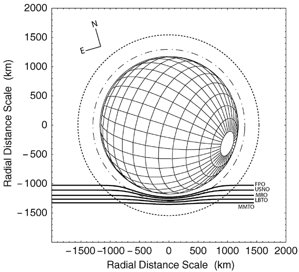
Figure 3. Occultation geometry from successful stations during the 2007 March 18 stellar occultation by Pluto: Pluto's south pole (IAU convention) is at the lower right. The light curves plotted were obtained from (south to north) the MMTO (6.5 m), LBTO (8.4 m), MRO (2.4 m), USNO (1.55 m), and FPO (0.32 m). The half-light radius in Pluto's shadow for this event, denoted by the dot-dashed line, was 1207 ± 4 km. The outer dotted circle indicates a 2% drop in the flux. Note that the central portion of the occultation, between the points where the MMTO curve drops below 0.95 flux, scans approximately 1200 km of Pluto's upper atmosphere.
Download figure:
Standard image High-resolution imageThe astrometric results from our simultaneous model fitting allowed us to establish the radius scale of the light curves. The resulting fitted solution yielded 1207 ± 4 km (Table 5) as half-light shadow radius (atmospheric radius at which the star light has dropped by 50% as measured in the occultation shadow, which is smaller than the corresponding radius in the atmosphere by a scale height of ∼60 km because of refractive bending) when fitted with the atmospheric parameters (λ and b) found in 2006. This shadow radius is consistent with the 1208 ± 9 km result measured in 2006 (Elliot et al. 2007) and indicates that the atmosphere has remained relatively stable since the cessation of the large increase in atmospheric pressure measured between the 1988 and 2002 observations.
6.2. Wave Structure
The MMTO visible light curve is displayed in Figure 4, mirrored and plotted against itself. Note that except for a few distinct features, the immersion and emersion sides of the light curve are almost identical. Thus, most of the individual oscillations are symmetric with respect to the light curve and also with respect to the planet's center. This symmetry indicates large-scale coherent structures—such as vertically propagating waves—in Pluto's atmosphere. As illustrated in Figure 3, the far immersion and emersion portions of the light curve (where the MMTO light curve drops below and then rises above 0.95 stellar flux according to Figure 2) probed regions separated by greater than 1200 km in Pluto's atmosphere. In addition, in order to be seen, distinguishable features in the light curve must be coherent through the refractive structure in Pluto's atmosphere encountered along the line of sight. We calculate (Elliot & Young 1992) this line-of-sight integration distance to be approximately 300 km. Thus, we interpret the structures causing the light-curve variations to be waves that are coherent across distances (1200 km and 300 km) that are sizable fractions of Pluto's atmospheric radius at the altitudes probed.

Figure 4. Highest S/N visible occultation light curve: the black line is a plot of the full resolution (4 Hz) light curve from POETS (Souza et al. 2006; Gulbis et al. 2008) on the 6.5 m MMT. This observation has a central wavelength of approximately 7400 Å ± 500 Å, based upon the response of the camera and the assumed stellar spectrum (M III). The red line is the same light curve reversed in time and overlaid on the original. Note the extremely close correspondence between the individual features on the extreme ends of the light curve. For example, the oscillations seen at 1330 s and 1520 s appear almost identical even though, with an occultation velocity of 6.8 km s−1, they occurred over 1200 km apart in Pluto's atmosphere. The most striking differences occur in the center of the occultation, where the atmosphere is probed most deeply, indicating that the higher-level structure is more coherent than at the lower altitudes.
Download figure:
Standard image High-resolution imageNote that hints of nonisothermal atmospheric structure have been seen before, but at smaller scales and lower altitudes. Structure in Pluto occultation light curves indicative of nonisothermal features was suspected for the 1988 occultation (Elliot et al. 1989) and definitively established for the occultation data obtained in 2002 (Elliot et al. 2003b; Sicardy et al. 2003; Pasachoff et al. 2005) and 2006 (Elliot et al. 2007), although for regions lower in Pluto's atmosphere than those probed by this event. Pasachoff et al. (2002) reported a striking correlation between light-curve spikes seen in 2002 from stations 120 km apart. However, the previous light curves were much lower in S/N than the data presented here and the features were sparse; hence, little could be said about the overall atmospheric structures that produced them.
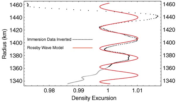
To pursue a more detailed solution than was provided by model fitting, we inverted (Elliot et al. 2003a) the MMTO visible light curve to establish detailed pressure, temperature, and number density profiles of the probed portions of the atmosphere. Figure 5 shows a plot of the inverted number density deviations of the immersion portion of the visible MMTO light curve from that for an isothermal atmosphere. Inversion of the emersion profile produces essentially the same structure as shown in Figure 5 with a slightly offset (∼17 km) radius scale. The astrometric solution indicates that we probed a region spanning approximately two scale heights, ranging from radii of 1340 km to 1460 km from Pluto's center. The density deviations were generated from the inverted number density profile by fitting it to a standard exponential function, and then dividing the inverted profile by this smooth exponential. This technique yields a density excursion plot (the black dotted line in Figure 5) that highlights the deviations of Pluto's atmosphere away from an exponential density profile. This profile reveals significant oscillations in Pluto's atmospheric density structure, which we attribute to vertically propagating atmospheric waves. Overplotted is an empirical model of a vertically propagating waveform with a wavelength of approximately 35 km at 1460 km radius. The wavelength of the data wave appears to decrease with decreasing altitude. This effect has been added as a simple linear term to the empirical model, with a lower wavelength of approximately 25 km at 1340 km radius. The density scale height of the atmosphere is approximately 54 km at these levels, so the waves persist through multiple e-folding scales in the area sampled. Also, note that the amplitude of the data wave increases with increasing altitude, a common feature of all vertically propagating atmospheric waves (Holton 2004).
Figure 5. Atmospheric number density from inversion of the MMTO visible light curve: the dots give the number density excursions of Pluto's atmosphere from a smooth exponential in the 1340–1460 km radius range. This excursion value is the result of the inverted number density profile being divided by the best-fitting exponential profile. The inversion covers Pluto latitudes from −47° at the top of the graph to −42° at the bottom. The lower portion of the inversion profile is shown in gray to emphasize the uncertainties resulting from small errors in background calibration. See Elliot et al. (2003a) for a discussion of this effect. The red line shows an empirical model of a vertically propagating wave, with a wavelength of approximately 35 km at 1460 km radius. Note that the wavelength decreases slightly with decreasing altitude reaching 25 km at 1340 km radius. The strong deviations between data and model in the uppermost portions of the inverted profile are due to the boundary condition imposed at the top of the inversion. The deviations in the lower atmosphere may indicate a breakdown in the coherent wave structures at lower altitudes, or that the zero-level calibration of the light curve is in error by a small amount (emphasized by the gray color).
Download figure:
Standard image High-resolution image
The effects of waves have been seen in occultation data from solar-system bodies such as Mars (Elliot et al. 1977; Barnes 1990) and Venus (Hinson & Jenkins 1995), although never before on Pluto. Observations of wavelike structure in the light-curve inversion profiles for large planets, such as those seen in the 1971 occultation of β Sco by Jupiter (Veverka et al. 1974), were examined by French & Gierasch (1974). They considered inertia-gravity, Rossby, and acoustic waves as possible sources of the β Sco inversion signatures, settling on inertia-gravity waves as most consistent with their data set. These inertia-gravity waves were later detected on Jupiter from Galileo probe data (Young et al. 1997). On small planets, undulations in the inverted atmospheric profiles from the light curve of a 1997 stellar occultation by Triton were attributed to "horizontal or vertical atmospheric waves," (Elliot et al. 2003a, p. 1041) but little effort was made to specify which waveforms were responsible. With the data set presented here, we are able to more deeply investigate the specifics of small-body waves and make estimates on the atmospheric limitations resulting from some of these possible wave sources.
Excitation of waves that are coherent over large distances requires a correspondingly large forcing mechanism—such as low-level winds encountering a properly oriented mountain ridge 1200 km long, or large-scale disparities in thermal heating. Inertia-gravity waves could produce the observed wave structures, an explanation that is addressed by analysis of the IR data from this event in a separate publication (McCarthy et al. 2008). Here we will consider Rossby waves (which can be present simultaneously with inertia-gravity waves), providing a possible explanation for this coherent structure. Rossby waves, without need for specific topography, naturally produce wave structures that are coherent over large fractions of the body's radius.
Rossby waves, identified in Earth's atmosphere in 1939 (Rossby 1939; Platzman 1968), are quasi-stationary (slowly-varying) oscillations that result from restoring forces that are dependent upon differences in the Coriolis force with changing latitude and, therefore, are less organized on a slowly-rotating body. However, Pluto's slow rotation must be weighed against its extremely tenuous atmosphere before discounting the significance of Rossby wave effects. The tenuous nature of the atmosphere, due to the Pluto's low gravity, is balanced by the slow rotation rate of the planet (and atmosphere) resulting in the possibility of stable wave structures.
For an upper boundary on the wind velocity associated with these wave effects, we can calculate the Rossby critical wind velocity Ucrit (horizontal) above which vertical propagation of Rossby waves becomes impossible. Following the derivation of Holton (2004), we find that the critical value of velocity grows with the horizontal extent of the waves (for stationary waves with respect to Pluto's surface):

In this equation, f is an average Coriolis parameter (2Ω sin ϕ, with Ω being the planet's angular velocity and ϕ being a given latitude) for the area probed by the light curve, β is the rate of change of the Coriolis parameter in the tangent-plane approximation, N is the usual buoyancy frequency, Hn is the density scale height, and k and l are the horizontal wave numbers. Here, we specify the horizontal wave numbers k and l in the line of sight and perpendicular directions, as we can make estimates of wave coherence in those directions from our occultation data. Table 7 gives all of these necessary values for the 2007 March 18 Pluto occultation, allowing us to calculate an upper limit for horizontal wind speed.
Table 7. Pluto's Atmospheric Parameters in 2007
| Parameter | Value |
|---|---|
| Half-light radius, rh (in atmosphere, km) | 1291 ± 5 |
| Rotational angular velocity, Ω (rad s−1) | 1.139 × 10⁻⁵ |
| Coriolis parameter at occultation mid-latitude, f | 1.972 × 10⁻⁵ |
| Density scale height at half-light radius, Hn (km) | 56.2 |
| Buoyancy frequency, N (s−1) | 1.390 × 10⁻³ |
Download table as: ASCIITypeset image
Since the maximum allowable wind speed in the presence of vertically propagating Rossby wave increases with decreasing wave number according to Equation (1), a reasonable upper limit would be to assume that the observed Rossby waves have a maximal wavelength given the atmosphere's size. Assuming that these variations are occurring at approximately 1400 km radius, we can use a wavelength of 1400π km in one direction (pole to pole) and 1400 (2π) cosϕ km in the other (for a latitude of ϕ = 60°), resulting in Ucrit = 3 m s−1. The assumption that the waves are standing waves of degree 1 (with wavelengths of maximum size) is justified (as an upper limit) since higher-order waves propagate less efficiently upward, so the upper limit is unlikely to be any lower. Indeed, on Earth, waves of higher than order 2 are rarely seen (Holton 2004). However, this fairly low upper limit makes Rossby wave stability problematic, requiring a very stable atmosphere to avoid disrupting the waves via wind shear.
We can establish a lower limit on horizontal wind speeds by rewriting Equation (1) and specifying the vertical wavelength from our inversion profiles. Again, using the vertical solutions derived by Holton (2004), we recast Equation (1) into an expression for horizontal wind speed, u, depending upon the vertical wave number, m:
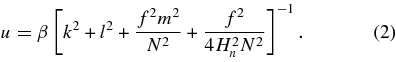
We then constrain the minima of the three wave numbers k, l, and m, using the occultation data. In Figure 5, the vertical peak-to-peak wavelengths are approximately 35 km. Line-of-sight coherence must be ∼300 km and perpendicular horizontal coherence must be at least ∼1200 km. Using these scales to establish wave numbers and substituting them into Equation (2) gives a lower limit on the velocity of less than 0.1 m s−1. Thus, if the observed vertical waves are to be interpreted as Rossby waves, they imply very stringent limitations on the possible wind velocities in this portion of Pluto's upper atmosphere.
7. DISCUSSION
The striking features in the upper atmosphere seen in Figure 5 could be attributed to effects other than Rossby waves. That the structure is due to some form of wave action is almost certain, given the detailed correlation of the light-curve structure between regions of Pluto's atmosphere many hundreds of kilometers apart. The tell-tale increase in amplitude with increasing altitude of the main oscillation is a significant indicator of vertically propagating waves. Internal gravity-wave signatures have been seen on the giant planets, and a discussion of a gravity wave solution to the current data has been examined by McCarthy et al. (2008).
How then does one distinguish between the various solutions? Further data from future occultations would certainly be helpful. Although the current data set covers a large portion of Pluto's atmosphere, Figure 3 indicates that we are primarily sampling equatorial latitudes. Given the dependence of Rossby waves on Coriolis effects, observation of a high Pluto latitude occultation at comparable S/N, as was obtained during the event observed in this study, could show a different picture.
Unfortunately, occultation geometries cannot be arranged to suit our observational needs. [Although observations from mobile platforms such as the upcoming Stratospheric Observatory for Infrared Astronomy (SOFIA) can provide more flexibility.] At Pluto's current orientation, polar occultation configurations are most likely to occur when Pluto approaches stationary points in its orbit with respect to an Earth-based observer. This north–south occultation line is therefore fairly rare, and no such events involving significantly bright stars are predicted for at least the next several years (McDonald & Elliot 2000).
Finally, it merits consideration whether Pluto's atmosphere is substantial enough to support stable or quasi-stable wave structures at these large wavelengths. One way to determine this is to look at the timescale for such density excursions to decay due to internal (macroscopic) diffusion processes. The timescale of this type of mixing is dependent upon the pressure scale heights of the atmosphere and the eddy diffusion coefficient (Atreya 1986). The eddy diffusion coefficient is generally measured empirically, but can be estimated as a product of the scale height and the mean velocity of the winds. Taking the range of velocities determined from the Rossby wave criteria discussed above yields a range of diffusion coefficients from 106 to 109 cm2 s−1. Using this range of values results in a wave collapse timescale ranging from almost half a year for the faster wind speeds to as little as 1 day at the lower limit. Although the timescale range is quite wide, reasonable wave propagation times are included in the upper portions of the range, giving us confidence in the possibility that stable wave structures indeed give rise to the observed density excursions. Alternately, considering molecular viscosity, the wavelength of 35 km is much greater than a particle mean free path in Pluto's atmosphere (<1 km). Thus, for Pluto, wave structures of this size need not break down due to diffusive or viscous processes.
8. CONCLUSION
We observed the 2007 March 18 occultation by Pluto from five stations throughout the western United States. Even with equipment and weather problems at two of the stations, useful data were successfully obtained at all stations. The data were reduced to light curves which were simultaneously fit for astrometric parameters of the event and atmospheric parameters of Pluto.
The atmospheric results of the model fits indicate that Pluto's overall atmospheric radius has stabilized for now after the dramatic increase between 1988 and 2002. The current atmospheric half-light radius of 1291 ± 5 km is consistent with the cessation of the pressure increase seen between 1988 and 2006 measurements.
The geometry of the event, coupled with the extremely high S/N from the two light curves from the MMTO on Mt. Hopkins (S/N = 340 and 490 per scale height, respectively, for the simultaneous observations in visible and IR wavelengths), reveals a picture of Pluto's atmosphere containing large-scale coherent wave structures. These structures extend at least 1200 km, and we model them as vertically propagating Rossby planetary waves. Assuming Rossby-wave propagation, we place upper and lower limits on atmospheric wind speeds at the atmospheric radii probed (1340–1460 km). The limits we find on horizontal wind speeds, less than 3 m s−1 at the 1400 km radius level, are significantly more constraining than prior upper limits based on possible atmospheric asymmetries observed in occultations (Person 2006). If the observed waves are interpreted as Rossby waves, these new tighter wind speed limits imply that if any atmospheric oblateness does exist, it is likely smaller than previously estimated, or the atmospheric oblateness arises due to something other than super-rotating winds—such as a distorted gravity field caused by a significant nonsphericity in Pluto's figure. An alternate explanation of the waves is presented in our companion paper in this issue. In either case, our results indicate that the New Horizons spacecraft, due to fly by in 2015, should find an active, dynamic atmosphere around Pluto.
We thank the engineering staffs of MMTO, LBTO, USNO, and MRO for their assistance. We especially thank Shawn Callahan (MMTO) for his extensive efforts allowing us to co-mount PISCES and POETS at the MMTO. We also thank Alan Plumb (MIT) for his theoretical insights and discussions. This work was partially funded by NASA Planetary Astronomy grants NNG04GE48G, NNG04GF25G, NNH04ZSS001N, NNG05GG75G, and NNX08AO50G to MIT and Williams College. Partial funding for MMTO observations was also provided by Astronomy Camp. Some of the observations reported here were obtained at the MMT Observatory, a joint facility of the University of Arizona and the Smithsonian Institution.