Abstract
Conditions and parameters affecting the range of bistability of the lac genetic switch in Escherichia coli are examined for a model which includes DNA looping interactions with the lac repressor and a lactose analogue. This stochastic gene–mRNA–protein model of the lac switch describes DNA looping using a third transcriptional state. We exploit the fast bursting dynamics of mRNA by combining a novel geometric burst extension with the finite state projection method. This limits the number of protein/mRNA states, allowing for an accelerated search of the model's parameter space. We evaluate how the addition of the third state changes the bistability properties of the model and find a critical region of parameter space where the phenotypic switching occurs in a range seen in single molecule fluorescence studies. Stochastic simulations show induction in the looping model is preceded by a rare complete dissociation of the loop followed by an immediate burst of mRNA rather than a slower build up of mRNA as in the two-state model. The overall effect of the looped state is to allow for faster switching times while at the same time further differentiating the uninduced and induced phenotypes. Furthermore, the kinetic parameters are consistent with free energies derived from thermodynamic studies suggesting that this minimal model of DNA looping could have a broader range of application.
Export citation and abstract BibTeX RIS

Content from this work may be used under the terms of the Creative Commons Attribution-NonCommercial-ShareAlike 3.0 licence. Any further distribution of this work must maintain attribution to the author(s) and the title of the work, journal citation and DOI.
1. Introduction
The lac circuit in Escherichia coli (E. coli) is one of the most well-studied examples of gene regulation, dating back to the classic experiments by Novick and Weiner in 1957 [1] and Jacob and Monod in 1961 [2]. Since then much has been learned about the system, including the effect of DNA looping on the effectiveness of the switch [3–6]. The lac operon controls the translation of genes necessary for the utilization of lactose. Three gene products are translated from the operon: β-galactosidase (LacZ) is responsible for cleaving the β-1,4 glycosidic bond in lactose to yield glucose and galactose, β-galactoside transacetylase (LacA) transfers an acetyl group to aid in lactose metabolism, and β-galactoside permease (LacY) is a membrane bound transporter protein, which actively imports lactose from the environment into the cell. A fourth constitutive protein, lac repressor (LacI), is coded for upstream of the lac promoter. This protein binds to the lac operators to inhibit transcription. When lactose enters the cell, some of it is converted to the lac inducer, allolactose. This binds to LacI, decreasing its binding affinity for the lac operators, which allow for more lac proteins to be translated. The lac circuit responds to glucose concentration by only producing the lac proteins when glucose is unavailable. During glucose starvation, cyclic adenosine monophosphate (cAMP) is produced which binds to the catabolite activator protein (CAP), allowing CAP to bind upstream of the lac promoter and recruit RNA polymerase (RNAP) to start transcription. Thus the lac switch acts as an AND gate to the signals 'low glucose' and 'high lactose,' only switching on when both are true. We are primarily concerned with the switch's response to the lactose signal.
Since producing more LacY leads to higher intracellular inducer concentrations, a positive feedback loop is set up allowing the cell to switch between two phenotypes: uninduced (lo), which produces a basal level of lac proteins and induced (hi), where the lac proteins are produced at their maximum rate. By increasing the extracellular inducer concentration the population of cells switch between uninduced, to a heterogeneous mixture of induced and uninduced, to all induced. Cells do not persist in intermediate states. These heterogeneous populations could enjoy a fitness advantage since some fraction of cells will always be prepared for changes in environmental conditions [7–9]. Although the lac system does not appear to be bistable except when a gratuitous inducer such as thiomethyl-β-d-galactoside (TMG) is used [10], this system is useful for studying the general phenomena of genetic switches. In the presence of minimal external glucose, LacI controls the production of messenger RNA (mRNA). The lac repressor binds to the main operator (O1) to prevent transcription. The binding affinity of LacI to the operator is controlled by the number of inducer molecules bound to the repressor. The lac repressor is a homo-tetramer, which can bind to two operators simultaneously: each dimer can bind to an operator individually. Each monomer can bind one inducer molecule for a maximum of four inducer molecules bound to the repressor.
The DNA sequence near the lac operon contains two auxiliary operators, which allow the local structure of the DNA to assume a looped conformation. DNA loops are ubiquitous in all domains of life as a regulatory tool, including transcriptional regulation in prokaryotes, enhancer sequences in eukaryotes, the lysis/lysogeny switch in phage λ, site-specific recombination, and DNA replication [11]. These loops occur when a protein or complex binds to two different sites along the DNA molecule, which could be separated by tens to thousands of base pairs. The regulatory effect can be understood as increasing the effective concentration of transcription factor near the binding site since the protein cannot diffuse away from the DNA unless both binding sites are dissociated [12]. All three operators O1, O2, and O3 are involved in the formation of DNA loops. Binding to either of the auxiliary operators, O2 or O3 only, is not sufficient to suppress transcription. However if both auxiliary operators are removed, the repression level is reduced by a factor of 100 [6]. Thus DNA loops appear to increase the ability of LacI to repress transcription.
A molecular mechanism for the induction of the lac operon both in the presence and absence of DNA loops was presented by Choi et al [3, 13]. In their study mutants were designed such that LacY was labeled with yellow fluorescent protein (YFP). Using the non-metabolizable inducer TMG, they were able to observe bistability in genetically identical populations of E. coli at concentrations of 40–70 μM of extracellular TMG. However using a population of mutants with both auxiliary operators removed, all cells deterministically switched into the induced state for concentrations of inducer as low as 20 μM. They argued that LacI must dissociate from both operators for induction to occur and that basal levels of LacY are due to partial dissociation of the DNA loop, leaving the operator downstream of the lac promoter free, allowing single transcripts to be produced infrequently before the loop reforms.
The lac switch has been a frequent subject of mathematical modeling. There have been many attempts to describe the system deterministically using chemical rate equations [10, 14–18] with varying levels of complexity. These models are successful in capturing much of the experimental behavior of the switch, such as identifying the number of phenotypes and the mean species numbers, however they cannot capture the full range of behavior of the lac system since they neglect the stochastic and discrete nature of chemical reactions. Indeed, it was shown in [14] that changing certain ratios of parameters that have no effect on a deterministic model, can have a strong effect on the corresponding stochastic model. It was also shown in [16] that the ranges of bistability predicted by deterministic modeling are much larger than what is realizable in a stochastic model. Deterministic models are also unable to compute switching times between states of induction since switching is a stochastic phenomenon. Stochastic models of lac have been developed to take this deficiency into account [13–15]. It is also possible to model genetic switches by not invoking a microscopic model, and instead focusing on the experimental copy number trajectories using the MaxCal method [19, 20]. This technique can provide a description of the intrinsic noise arising from small copy numbers [21–23]. Theory developed in general for stochastic gene expression [24–31] can also provide a reasonable description of the system. However, none to our knowledge attempt to include the effect of DNA loops on the range of bistability and switching rates.
Here we present a stochastic treatment of a gene–mRNA–protein model of the lac operon in E. coli interacting with extracellular inducer that includes transitions to looped DNA states. We develop a novel combination of the finite state projection (FSP) [32] and geometric burst approximation (see below) to render the chemical master equations (CMEs) computationally tractable and show that rare random loop dissociation events are responsible for the lo→hi phenotypic transition. Our results show that the process of induction in the lac operon is preceded by the total dissociation of the DNA loop. We show that the microscopic mechanism of switching in the three-state model is fundamentally different than the mechanism in a model without DNA looping. The looped state alters the switching dynamics such that fast switching times between the metastable states are possible while minimizing noise within those states. A model without the looped state shows a minimal range of bistability below 20 μM of external inducer concentration, whereas the three-state model shows the full range of bistability as observed in experiments [33].
2. Model
In this work, we consider two models for gene expression from the lac operon. The first model is the standard two-state model of gene expression in which the two states represent the DNA's transcriptional state, either repressed or active. The second model adds an additional third state to account for the possibility of a potentially long-lived looped state with different transcriptional properties. Figure 1 shows a schematic representation of the two models. All parameters are defined and values given in table 1.
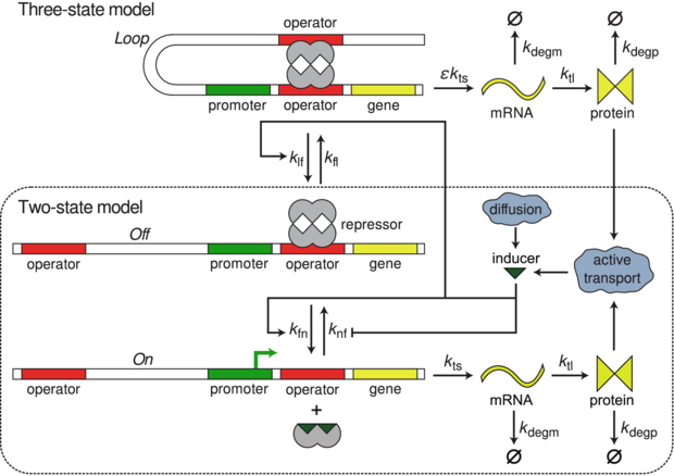
Figure 1. Cartoon schematic of the three-state model of the lac circuit. The two-state model is exactly the same except without the Loop state. There are three states controlling the transcriptional state of the switch: On producing transcripts at the nominal rate with O1 free, Off where no transcription is possible due to O1 being bound to LacI, and Loop which is a coarse-grained state representing any of the possible looped states and singly bound DNA/repressor states which do not inhibit transcription. This state models the proposed phenomenon of transcriptional leakage in which fluctuations of the repressor/DNA complex can allow rare transcription events to occur while in an otherwise looped conformation [3]. The switch can be induced by adding external inducer to the environment. The inducer is then transported into the cell via diffusion and active transport by lactose permease where it binds to the lac repressor, decreasing its binding affinity for the lac operators. This decreased affinity allows the lac repressor to fall off and allow RNA polymerase to bind and transcribe mRNA. The system now transitions from Loop through Off to On where transcripts are produced at a higher rate, setting up a positive feedback loop where more transporter protein is translated.
Download figure:
Standard imageTable 1. Selected parameter set from mean of parameter search. The fixed parameters were taken from [33] or extracted from fits to data therein.
| Symbol | Description | Value | Units |
|---|---|---|---|
| Selected from parameter search | |||
| k0lf | Loop→Off rate at zero inducer | 1.45× 10⁻⁴ | s−1 |
| k1lf | Loop→Off rate at saturating inducer | 3.31× 10⁻³ | s−1 |
| Hlf | Hill coefficient for Loop→Off | 3.12 | |
| Ilf | Hill concentration for Loop→Off | 3940. | μM |
| kfl | Constant Off→Loop rate | 3.83× 10⁻³ | s−1 |
| Fixed parameters | |||
| k0nf | On→Off rate at zero inducer | 5.04× 10⁻² | s−1 |
| k1nf | On→Off rate at saturating inducer | 5.04× 10⁻⁴ | s−1 |
| Hnf | Hill coefficient for On→Off | 1. | |
| Inf | Hill concentration for On→Off | 17.4 | μM |
| k0fn | Off→On rate at zero inducer | 6.30× 10⁻⁴ | s−1 |
| k1fn | Off→On rate at saturating inducer | 3.15× 10⁻¹ | s−1 |
| Hfn | Hill coefficient for Off→On | 1.67 | |
| Ifn | Hill concentration for Off→On | 5680. | μM |
| kts | Transcription rate | 1.26× 10⁻¹ | s−1 |
| ktl | Translation rate | 4.43× 10⁻² | s−1 |
 |
Leakage factora | 8.33× 10⁻⁴ | |
| kdegm | mRNA degradation rate | 1.11× 10⁻² | s−1 |
| kdegp | LacY degradation rate | 2.10× 10⁻⁴ | s−1 |
| kit | Turnover number for active transport | 1.20× 101 | s−1 |
| kid | Rate of LacY diffusion | 2.33× 10⁻³ | s−1 |
| across membrane | |||
| Km | Michaelis constant for active transport | 400. | μM |
| Vcell | Volume of cell | 8.00× 10⁻¹⁶ | L |
aEstimated from [3]
2.1. Two-state model—no DNA looping
The two-state model contains two transcriptional states for the DNA, Off and On where the operon is transcriptionally inactive and active, respectively. DNA looping in not possible in this two-state model. When the operon is in the On state, transcription proceeds as a first order reaction

Protein (Y) is translated at a rate that is proportional to the mRNA (m) copy number

and protein and mRNA degrade at a rate proportional to their respective abundances
Due to interactions between the lac repressor and inducer molecules, switching between the active and inactive transcriptional states occurs at a rate dependent on the inducer concentration inside the cell,
The switching rate functions kfn([I]) and knf([I]) are determined by the microscopic interactions between the repressor and inducer. It was previously shown [33] that a particular microscopic model for these interactions gave rise to switching rates that were first-order for a given constant inducer concentration and with functional dependencies on inducer concentration that could be well-described by Hill-like functions. We fit the simulation data from [33] (see supporting information section S1 available at stacks.iop.org/PB/10/026002/mmedia) to the functions
and
and obtain Hill-like expressions for the rate functions in our model in terms of internal inducer concentration. Here the parameters k0x and k1x determine the minimum and maximum transition rates, Ix is the internal inducer concentration that the transition rate is  , and Hx is the Hill coefficient, which is proportional to the slope at [I] = Ix.
However, including the inducer as a separate species would dramatically increase the complexity of the model. Instead we express the transition rates in terms of the number of LacY proteins in the cell membrane,
Consider that inducer (I) can enter the cell either through passive diffusion from the environment (with constant concentration [I]ex),
or through active transport by the LacY protein (modeled using irreversible Michaelis–Menten kinetics),
If we assume that inducer responds very quickly to a change in the LacY concentration, we can solve for the steady-state concentration of internal inducer as a function of the LacY and external inducer concentrations:
with
Substituting equation (11) into equations (6) and (7) we obtain expressions for kfn(Y) and knf(Y) with a little algebra.
2.2. Three-state model—with DNA looping
Since the lac operon has three operators to which LacI can bind, the transcriptional states are more complicated than On and Off alone. The simplest modification to the two-state model to handle this complexity is to add a third state—Loop—that describes the operon when it is in a looped conformation with the repressor. It was hypothesized that in a looped conformation the LacI–O1 binding can fluctuate allowing RNAP to bind and transcribe while O1 is unoccupied with LacI nearby [3]. We introduce the Loop state to model this effect. This third state should not be interpreted as a specific conformation of the operon/repressor complex. Instead it should be understood as a coarse-grained state that represents all DNA/repressor looped conformations (O1–O2 and O1–O3) as well as bound conformations in which transcription is not repressed (O2, O3, or both bound). This state allows for the slow leakage of transcripts. We model this leakage by allowing transcription from the Loop state at a rate times the normal On transcription rate by adding the reactions
and

to our model. The leakage factor is conditional probability to have repressor bound to O2, O3, or both O2 and O3 while in the Loop state. The schematic representation of the two models are shown in figure 1. This three-state model is similar to another three-state promoter model, which has been investigated recently [34]. This work focused on the stochastic mutual repressor model and described the state of the operators using three transcriptional states. Their methods would be difficult to implement for our models due to the noise in the translation rate arising from fluctuating mRNA abundance.
We estimated from [3]. They measured the distribution of YFP counts in a mutant with the lac circuit modified to disable positive feedback while allowing DNA loops to form. This experiment was conducted by replacing LacY with a Tsr-YFP fusion protein, which also localizes in the cell membrane, but cannot import allolactose into the cell. These distributions were well-described by a gamma distribution parameterized by the burst rate a and the burst size b. This approximate result was derived from a gene–mRNA–protein model with one transcriptional state [26]. The burst rate a ≡ kts/kdegp can be interpreted as the number of transcripts produced per cell cycle and the burst size b ≡ ktl/kdegm refers to the average number of protein transcribed from a single mRNA. The burst rate and the burst size were measured for TMG concentrations between 0 and 200 μM and found to be relatively constant over this range: 0.34 < a < 1.25 and 1.29 < b < 2.59. We used this measurement to estimate that 5.7 × 10⁻⁴ < < 2.1 × 10⁻³ and assumed = 8.3 × 10⁻⁴ for our model. The two transcription rates kts and kts are responsible for the different burst sizes observed in [3]. 'Small' bursts of transcription occur due to leakage whereas 'large' bursts occur due to full dissociation of the complex (Loop→Off→On).
Since the On↔Off switching rate functions were well-described by a Hill function, we assume that the Loop to Off rate function could also take that form. Thus
We will assume that the Off to Loop rate is constant in inducer concentration, since transitions into the looped state must occur via thermal fluctuations that take the singularly bound inducer/DNA complex into a conformation in which the unoccupied binding site on the lac repressor can reach a free operator. It is not possible to determine these switching rates directly from the data available from the literature, so we search the parameter space to determine for which values of these parameters the system exhibits the desired response. Of the parameters presented in table 1, only the five parameters describing the constant Off→Loop rate and the Loop→Off Hill function (15) are predicted. The remaining parameters are taken from the literature [3, 14, 33].
2.3. Deterministic and stochastic representation
The deterministic rate equations for mRNA and LacY abundance are
where x and y are (continuous) concentration variables for mRNA and LacY respectively. Here we have defined the total transcription probability,
where the Pz(y) functions are the probability to find the system in the transcriptional state z at fixed protein abundance y and are computed simply from considering the steady state of a Markov process consisting of the three transcriptional states alone. This process is represented by
which at steady state is governed by the master equation
whose normalized solution is


with  , and y is computed from [I] by (11).
To investigate the fixed points of equations (16)–(17), we take the time derivatives to be zero and solve for y to get
where
is approximately the mean population of the induced state. For a set of parameters exhibiting bistability over some range of [I]ex, the form of  allows the dynamical system to exist in three distinct phases. For low values of [I]ex, the system has a single stable fixed point at nlo corresponding to the uninduced phenotype. For high values of [I]ex the system has a single fixed point at nhi corresponding to the induced phenotype. For intermediate values of [I]ex, there is a range in which the dynamical system has three fixed points: two stable fixed points nlo and nhi and an unstable fixed point n0. This external inducer regime corresponds to a heterogeneous population containing both phenotypes. The locations of these fixed points are not fixed, but can change with the inducer concentration. For the transcription state transition functions considered here, (24) is generally not solvable analytically due to the form of transcriptional state rate functions used.
The probability to be in a particular transcriptional state at a specific mRNA and protein abundance can be determined by solving the CME for the system [35]. These equations govern the time evolution of the probability, Psmn, to find m mRNA molecules and n proteins, when being in transcriptional state s. Writing out the transcriptional states explicitly we have
where  are step operators that increment/decrement the mRNA index (M) or protein index (N) by i. The rates ktl, kdegm, and kts,kdegp are the mRNA birth and death rates and protein birth and death rates respectively. The functions knf(n), kfn(n), kfl, klf(n), are the transcriptional state switching rates for On→Off, Off→On, Off→Loop, and Loop→Off.
3. Methods
The CMEs (26)–(28), being two-dimensional, are unsolvable analytically. An approximate solution was derived [25] for the two-state system without feedback in the limit
however this approximation is unfeasible here since they used a generating function technique which is not applicable when the feedback functions are non-polynomial. A solution in this same limit is also possible for the two-state system with arbitrary feedback functions. This solution was derived using the Wentzel–Kramers–Brillouin (WKB) approximation [36] to the CME, which allowed for the accurate calculation of the mean switching times between the metastable states [24]. We attempted a similar solution to our three-state problem by taking the CMEs (26)–(28) in the quasi-stationary approximation and applying the WKB ansatz  . This substitution yields a stationary Hamilton–Jacobi equation to leading order in
  with Hamiltonian
Here the species numbers are scaled by the system size (25),  ,
,  , pi is the momentum conjugate to coordinate i (pi = ∂iS) and
in units where kdegp ≡ 1. However, due to the fast switching times between the metastable states (see below) the WKB method is inapplicable here since it requires that the escape time from the metastable state be exponentially large in the typical system's size, see e.g. [37–39].
Direct numerical solutions will be computationally intensive and not feasible for optimization due to the dimensionality of the resulting system of ODEs. Reasonable values of maximum protein number and maximum mRNA number lead to a system of 450 000 equations. In order to make progress we must employ some method of approximation.
3.1. FSP solution of CME using the geometric burst approximation for mRNA
In bacteria the ratio γ is typically large. We can use this fact to eliminate the mRNA degree of freedom from the CMEs. It is well-known that it is not sufficient to replace the mRNA dynamics with the average mRNA abundance while studying the switching times [24, 40, 41]. Transcriptional noise will lead to increased noise in protein abundance, which will affect the switching rates between induced and uninduced phenotypes. Another option would be to apply the quasi-steady-state approximation to the CMEs [42], however due to the stochastic switching of the transcriptional states, the transcription rate is not constant and thus the mRNA distribution is not at steady-state. We need to apply a different tack.
To remove the mRNA degree of freedom while still accounting for transcriptional noise we will exploit the fact that the number of protein molecules translated from a single mRNA is distributed geometrically. In the limit γ → ∞ an effective CME can be written without mRNA dependence by assuming that translation occurs in bursts with sizes that are geometrically distributed [43]. Figure 2(b) describes this pictorially. Since the probability that a single mRNA molecule is translated n times before decaying is
the translation terms in (26)–(28) can be rewritten as
and we can drop the transcription terms, mRNA degradation terms, and mRNA indices. For example, consider the one-state model with the master equation
This transforms to
All mRNA dependence is removed and now the translation term is that of a multi-step process where for a protein state n, transitions into that state can come from any protein abundance state from 0 to n − 1. Transitions out of the state n for translation can go to any state greater than n. These transitions are accounted for by the 1 in the translation term since the geometric distribution is normalized and the probability for a single transcription is Ptl. The protein decay term is not affected by this manipulation. This substitution is an adiabatic approximation that assumes that all mRNA is created or degraded between each protein reaction. This approximation is only valid when there is a large difference in time scales between the mRNA and protein dynamics. For E. coli, γ ≈ 53 based on degradation rates assumed for our model (cf table 1). This ratio is sufficient large that the mRNA and protein dynamics are well-separated. For the three-state model, this approximation reduces the dimensionality of the underlying system of equations by a factor of mmax (≈50) and significantly decreases the computational time. Analytically, this reduces (26)–(28) to a single dimension. A similar geometric bursting approximation for mRNA was used in a previous calculation [44] however only the average and variance of the protein abundance at steady-state could be calculated. To compute the full probability distribution of protein abundances and the switching rates between the induced and uninduced phenotypes a different method of solution must be employed.
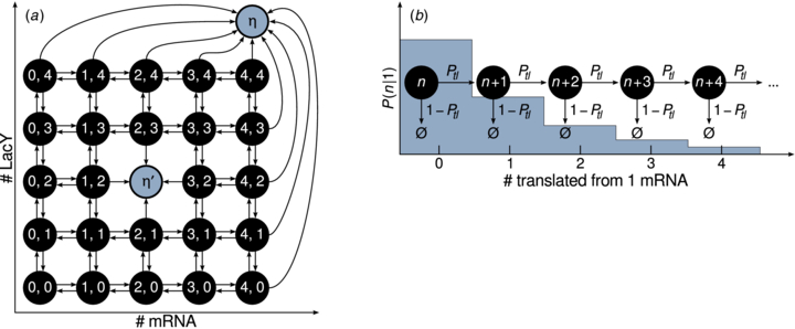
Figure 2. (a) Finite state projection. Consider a gene–mRNA–protein model having only one transcriptional state. The FSP method truncates the state space, eliminating states that are not well-populated. Here we have chosen the projection n, m < 5. Transitions that would lead to n or m = 5 are rerouted to the sink η. As the equations are evolved in time, the total probability accumulated in η is monitored. If η increases past a threshold, the calculation is restarted with a projection including more states. This technique can also compute mean first passage times. The state n = 2, m = 2 is replaced by a sink state η' from which no probability can flow out. The accumulated probability in η' is the distribution of first passage times to n = 2, m = 2. (b) Geometric burst approximation. Each time a mRNA is transcribed, it can be translated increasing n by 1 or be degraded and become unable to be transcribed further. This process leads to a geometric distribution of protein translated from a single mRNA.
Download figure:
Standard imageWe numerically integrate the CMEs using the FSP to compute an approximate solution [32, 45]. This method is significantly faster than directly sampling the CMEs using the stochastic simulation algorithm (SSA). Computational time can be over 100 times shorter using this method compared to using the SSA with a sufficient number of realizations to be comparable to the error achieved from the FSP. To achieve this level of performance, this method truncates the state space at copy numbers that are not expected to be well-populated. The error due to the truncation is controlled adding fictitious states denoted sinks that accumulate probability that leaves the projection. Any transitions to states outside the projection are rerouted to these states. For example see figure 2(a), where the sink states are labeled η. The total probability lost due to the projection is the sum of probability in the sinks, which estimates the total error due to the truncation of state space. To find the optimal size of the projection, the system of ODEs is integrated while monitoring the accumulated probability in the sinks. If the sink probability increases past a threshold, the calculation is restarted with a larger projection space. The method for increasing the projection space depends on the type of problem being considered, for examples see [32, 46, 47]. For our simple 1D CME, we choose for our state projection ![$n\in [0,\alpha \mathcal {N}]$](https://content.cld.iop.org/journals/1478-3975/10/2/026002/revision1/pb445050ieqn37.gif) where α is 1.25 initially and is increased when the calculation must be restarted.
where α is 1.25 initially and is increased when the calculation must be restarted.
Writing the CMEs in matrix form would lead to a large non-sparse matrix due to the tail of the burst distribution, because each state (n, s) can transition to (m, s) where  . Considering protein burst reactions alone, this situation leads to a block diagonal matrix where each of the three blocks are lower triangular. This problem can be solved by truncating the geometric series used in the burst approximation leading to a generator with a band structure. Any transitions from translation where the change in protein number is larger than a threshold are rerouted to a sink. Error due to the truncation of the geometric expansion is monitored by watching the accumulation in this sink. We found that 120 terms in the expansion were sufficient to achieve a total error of less than 10−7. Since (26)–(28) are not explicitly dependent on time, we integrated the equations using an off-the-shelf matrix exponentiation package [48].
3.2. Mean first passage times
We are interested in the mean switching rates between the induced and uninduced metastable states. These rates can be computed from the mean first passage time (MFPT) for the system to evolve from a stable fixed point of the deterministic rate equations (24)—either nlo or nhi—to the unstable fixed point n0. Although there are elegant techniques available for estimating the stability of metastable states [49–51], we can compute these rates quickly and accurately using the geometric burst approximation coupled with the FSP. We compute the MFPTs by adding an additional sink at n0, and integrating the equations with the initial condition that the copy number probability at the initial stable fixed point is unity [52].
The probability accumulated in this sink, η(t), is the cumulative distribution function (CDF) of first passage times. Aside from an initial transient period, the time evolution of η(t) is well-described by η(t) = 1 − e−t/τ. We could then integrate the equations out to a time tf where η(tf) ≈ 1 and extract the MFPT τ by curve fitting. To save computational resources we use a different approach which does not require the equations to be integrated to tf.
The mean of a distribution can be computed from its CDF by integrating the complementary CDF over its full domain. We will use this fact to estimate the MFPT by integrating over the known part of the full domain and adding to this value an estimate of the rest of the integral. At each time ts during the integration of the CMEs, we integrate the complementary CDF 1 − η(t) numerically up to the current time step ts and estimate the contribution from the integral from ts to ∞ by assuming the complementary CDF decays exponentially for times greater than ts. Thus at each time step we compute
where
We stop when the change in τ(ts) per time step is less than a threshold:
For a tolerance of total error less than 5× 10⁻⁴, the algorithm requires ≈300 steps to converge.
3.3. Calculating the range of bistability
We define the macroscopically bistable range to be the range of inducer concentrations where the probability to be either lo or hi is greater than 10%. We find this range for a given set of parameters by first finding the range of external inducer concentrations that lead to three fixed points in the deterministic rate equations by counting the roots of (24). This range of concentrations is then searched, looking for where the probability to be in the induced state
is 0.1 and 0.9. Here τx is the MFPT out of the phenotype x. We then search this bistable range for the concentration that either induction state is likely (P(hi) = 0.5), and ensure that the rate at the candidate concentration is greater the minimum acceptable value. The search is performed using the MFPTs computed from geometric burst/FSP method using standard root finding algorithms.
3.4. Sampling the CME using the stochastic simulation algorithm
To test our results from the FSP calculations, we used the SSA [53] to compute the probability distribution functions (PDFs) and MFPTs. To look at the microscopic dynamics of switching events, the trajectories from the SSA simulations were segmented into induced, uninduced, and switching sections using thresholding heuristics that allow for arbitrarily long switching trajectories.
The heuristics first mark regions of the trajectory as lo if the protein number is lower than the unstable fixed point, and hi otherwise. An acceptable switching event is a segment of time t0 long that does not leave lo (hi) followed by an intermediate segment less than δtmax long that fluctuates between the two states followed by a segment of time t0 long that stays in hi (lo). The lead-in and lead-out times will not affect the results since the model is Markovian. We chose t0 = 10 cell cycles. The maximum switching time δtmax was chosen so greater than 99.9% of the trajectories with long enough lead-in and lead-out times were accepted. The necessary δtmax depends on the particular parameter set but was generally of the order of 50 cell cycles.
4. Results
4.1. Looping parameters that reproduce lac bistability
A primary goal for the work is to determine if a minimal three-state model is able to recover the full range of bistability that was experimentally observed for the lac circuit with looping, compared to the behavior observed for the circuit where looping was prohibited. However, the model's looped state represents a coarse-grained state composed of many different microscopic states and no experimental data regarding microscopic transition rates are known. We therefore searched the space of all possible parameters related to the loop state to characterize how its addition changes the behavior of model. The Off→Loop transition has a single parameter kfl and the Loop→Off transition function has four parameters: k0lf, k1lf, Ilf, and Hlf. We randomly choose parameter values from this five-dimensional space while keeping all other model parameters fixed and tested the model's bistability properties.
To limit the size of the search, we bounded the parameter space such that only biologically reasonable parameter sets were sampled. The Off→Loop transition models the physical process of forming a DNA loop. If it is too slow to observe, the three-state model reverts the two-state model so we set the minimum rate of kfl to be one event per 100 cell cycles. Likewise, loop formation requires the binding of a repressor–operator complex to a second operator and must be slower than repressor binding, so we set the maximum of kfl to be one-half the rate of repressor binding, k0nf/2.
For the Loop→Off transition Hill function klf(n), the parameter Ilf determines the approximate inducer concentration at which the transition rate will start to increase, i.e. at what inducer concentration the loop starts to become destabilized. We bounded this parameter such that the denominator in (15) is  for inducer concentrations between 1 and 100 μM. This bound ensures that the transition rate function is able to switch between its low and high ranges over the experimentally relevant range of inducer concentrations. If Ilf was too large or too small, klf(n) would be effectively constant over the full range of LacY abundances and not provide feedback. The Hill coefficient Hlf determines the sharpness of the response and was restricted to be between 2 and 4 since inducer–repressor binding is cooperative with four binding sites. An in vitro study of DNA loop stability for the wild-type lac operon reported the mean lifetime of the loop to be on the order of the cell cycle [54]. In light of this observation, for the minimum transition rate k0lf (in the absence of inducer) we generously bounded this value by setting the minimum rate for the search to be one dissociation per ten cell cycles and the maximum rate to be one-half of the repressor unbinding, k0fn/2, since by definition loop dissociation must be slower than repressor unbinding. The maximum transition rate k1lf (in the presence of saturating inducer) was restricted to be faster than twice the zero inducer rate k0lf but slower than 100 events per cell cycle.
We scanned 125 113 unique parameter sets by uniformly drawing a random value for each parameter from the above ranges. For each set we calculated the range of macroscopic bistability, defined at the low end by the inducer concentration where 10% of the steady state population is induced and at the high end by the inducer concentration where 90% of the population is induced (see section 3.3). Whereas the two-state model exhibits bistability near 10 μM (10.1–10.9 μM), the three-state model can produce bistability at inducer concentrations anywhere from 10.6–518 μM for sets of parameters constrained to the range above. Additionally, the range of macroscopic bistability for the two-state model is very small, 0.8 μM, while the addition of a third state can produce much wider ranges, up to 300 μM. As the overall switching rate to Loop decreases, the bistability range increases on average.
For each set we calculated the mean switching time at the inducer concentration where 50% of the steady-state population is uninduced and 50% is induced. At this concentration the time to switch to lo or to hi is identical and we use this time (τ50%) as a measure of a parameter set's characteristic switching time. For the two-state model, τ50% was 55 cell cycles, but with the three-state model τ50% values could be obtained anywhere from 26–9.5× 10⁵ cell cycles. Decreasing Ifl has the effect on average of increasing the switching time τ50% (see supporting information section S3 available at stacks.iop.org/PB/10/026002/mmedia).
Having performed a parameter search for the looped state, we then selected for further study only those parameter sets that reproduced the range of bistability seen in one experiment [3]. A parameter set was deemed acceptable if its range of bistability contained the range 50–60 μM and τ50% was less than 100 cell cycles. Approximately 0.9% of the random samples satisfied these criteria. Figure 3 shows how the accepted parameters were distributed in the search space.

Figure 3. Two-dimensional distributions of parameter values in sets with bistability ranges including 50–60 μM. Lighter areas indicate greater density. A large range of parameter sets exhibiting bistability with fast switching rate were found. The dot marks the mean of the distribution. This parameter set is investigated in later figures.
Download figure:
Standard imageThe absolute value for several of the parameters appear to be unimportant to the switching properties. The Hill coefficient Hlf and the basal Loop→Off rate k0lf are well-distributed within their allowed ranges. Likewise, the Off→Loop rate kfl is uniformly distributed below 45 cell cycles. On the other hand, the inducer transition concentration Ilf and the maximum Loop→Off rate k1lf are more likely to take on values in certain ranges of the search space, high and low, respectively.
Some parameters showed a degree of mutual dependence. The basal Loop→Off rate k0lf and the Off→Loop rate kfl have a strong linear dependence (r2 ≈ 0.6). Together with their uniform distribution, this dependence suggest that the total fraction of the time spent in the looped state in the absence of inducer, which determines the basal permease copy number, is an important property for switching, but the rate of cycling between the looped and unlooped states is relatively unimportant.
The inducer transition concentration Ilf and the maximum Loop→Off rate also appear to be dependent. All of the accepted sets fall above a convex region of the Ilf–k1lf phase space: k1lf ≲ Ilf4. If the maximum Loop→Off transition rate is high, then the transition concentration must also be high and if the transition concentration is low the Loop→Off transition rate must be low. A similar but less pronounced dependence is seen between the maximum Loop→Off rate and the Hill coefficient Hlf. This dependence is simply because there appears to be a maximum Loop→Off rate. When Ilf is large, klf(n) will not be able to reach its saturating level so values of k1lf larger than the maximum rate can be used.
The distribution of calculated switching properties for the accepted parameter sets is shown in figures 4(a)–(e). The onset of bistability, the external inducer concentration necessary for 10% induction probability can begin, as low as 30 μM and can last through 120 μM. The width of the bistable range can be from 20–80 μM. τ50% values fall between 25–100 cell cycles. The properties of LacY in these cells is also of interest. The uninduced states were centered at zero LacY for all acceptable sets and the induced state means were found at 2350 ± 10.

Figure 4. Distributions of calculated values from the set of parameters with bistability. The dotted line marks the values computed from the selected set in figure 3. These are distributions of inducer concentrations at (a) 10%, (b) 50%, and (c) 90% probability to be induced, (d) extent of the bistable range, (e) metastable state lifetimes at 50% induction probability, and (f) average LacY count in the induced state.
Download figure:
Standard imageWe tested the sensitivity of the model to changing the leakage factor . Over the likely range of from 5.7× 10⁻⁴ to 2.1× 10⁻³, the range of bistability only changed from 23.0 to 22.75 μM. The switching lifetime τ50% only changed from 54.7 to 53.8 cell cycles.
4.2. Details of a representative parameter set
We chose as a representative parameter set the mean of the acceptable parameter set distribution since that approximates the centroid of the hypervolume that encloses all acceptable parameters. In figure 3 this parameter set is indicated by a white point, the details of these parameters are enumerated in table 1, and the transcription state transition functions are plotted in figure 5. The PDF computed for this parameter set and the two-state model are shown in figure 6 compared to the PDF computed from the SSA. The combined FSP and geometric burst approximation predict the probability distributions with a high degree of agreement. The total probability lost from transitions out of the projection was less than 10−4, and the probability lost from truncating the geometric distribution was less than 10−7. The deviations of the FSP PDF from the SSA PDF are due to the adiabaticity assumption of the geometric burst approximation, not from probability loss from truncation. A numerical solution of the CMEs for the two-state model with explicit mRNA dependence showed exact agreement with the simulated distribution (see supporting information section S2 available at stacks.iop.org/PB/10/026002/mmedia) but with drastically increased computational cost.

Figure 5. Comparison of the transcriptional state switching functions used. (a) Functions used in the two-state model at [I]ex = 10.5 μM. (b) Functions computed using values from the mean of the parameter search distribution for the three-state model at [I]ex = 55.3 μM. The function  is the extracted switching function from an effective two-state model built from the results of the three-state parameter search.
Download figure:
Standard image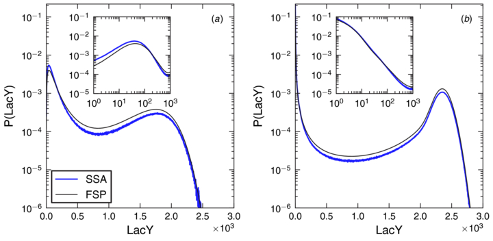
Figure 6. Protein number PDF computed from simulation (SSA) and the geometric bursting approximation (FSP) for (a) the two-state model and (b) the three-state model. The inducer concentration was chosen such that the system was equally likely to be in either induction state. The inset shows a closer look at the uninduced state distribution on a log–log scale. Slight deviations from simulation are due to the geometric burst approximation. Computations of the PDF including explicit mRNA dependence (not shown) fit the simulation identically.
Download figure:
Standard imageThe dependence of induction state lifetime on the external inducer concentration is generally exponential as shown in figure 7. Since changing the inducer concentration just affects the effective transcription rate, this functional dependence is in agreement with what is known about the dependence of switching rates in genetic networks [40]. This parameter set is bistable within the external inducer concentration range of 42–66 μM using 10% minority as the bistability metric. The switching time at equal induction probability is 63 cell cycles. For the two-state model, the bistability range was 10.1–11.0 μM with a switching time of 52 cell cycles. These values are in agreement with the results presented in [3] however the bistability of the non-looping mutant was only tested down to 20 μM external inducer so a transition from the induced phenotype to uninduced could not observed.
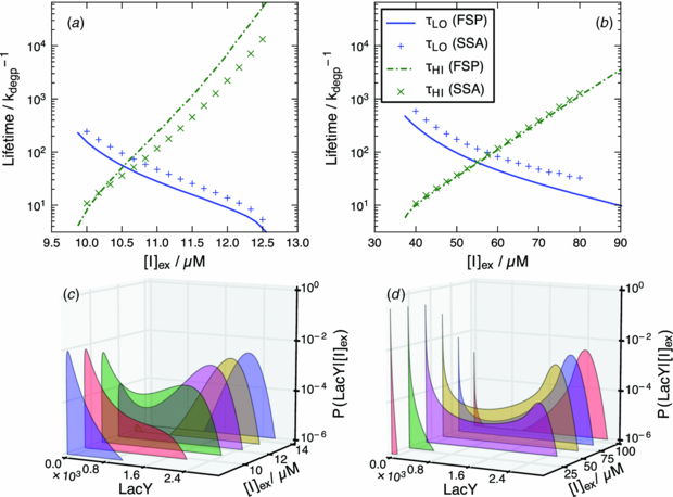
Figure 7. Comparison of lo and hi metastable state lifetimes for both (a) the two-state model, (b) the three-state model computed via simulation (SSA) and using the geometric burst approximation (FSP) reported in cell cycles. The deviations from simulation are due to the geometric burst approximation. The point where the two lifetime functions cross is the equal probability concentration, and the lifetime here sets the scale for switching times. Dependence of PDFs on external inducer concentration for (c) the two-state model and (d) the three-state model computed using the geometric burst approximation.
Download figure:
Standard imageThe mean protein number in the uninduced states appear to be in agreement with experiment. This parameter set exhibits an uninduced state centered at 0 LacY whereas the two-state model has an uninduced state centered at 41. The location of the modes is in agreement with [3] since they showed for mutants unable to produce permease that the LacY distribution was centered at 0 for low inducer concentrations and the LacY distribution for mutants that cannot form DNA loops or produce permease was centered around 75. They did not report copy numbers for the induced state, however we found that adding DNA looping resolved the differences between the induced and uninduced states by moving the induced maximum from 1778 to 2351 and decreasing the width of the distribution by a factor of 2.7.
4.3. Microscopic dynamics of induction state transitions
To investigate how the system transitions between the two phenotypes, we plotted protein and mRNA abundance histograms at regular time steps during a switching event in figure 8. We computed multiple trajectories using the SSA and searched them for segments in which the system switched between metastable states. All segments were then translated in time such that the first transcriptional state change event before switching is at t = 0.
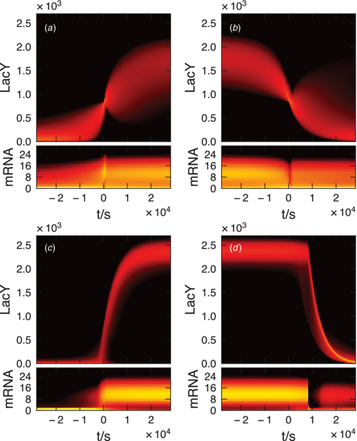
Figure 8. Distributions of protein and mRNA abundance as a function of time for (a) the two-state model transitioning lo→hi, (b) transitioning hi→lo, (c) the three-state model transitioning lo→hi, and (d) transitioning hi→lo. Induction and uninduction events in the two-state model are driven by protein number fluctuations, however in the three-state model fluctuations of the transcriptional state drive the switch, leading to quasi-deterministic behavior.
Download figure:
Standard imageFor the lo→hi transition, the three-state model shows quasi-deterministic switching behavior with an average switching time of 2.9 cell cycles. The duration and shapes of the protein trajectory during a switching event are all uniform. The two-state model does not exhibit this behavior. Instead the transitions are stochastic and irregular. The reason for this behavior appears to be that the three-state model stays in the Loop state in the uninduced phenotype and very rarely switches into Off. Prior to switching the mRNA population increases leading to more frequent bursts of protein, which can carry the system from the Off transcriptional state into On. Once On is reached switching back to Off is rare, leading to the deterministic switching behavior.
The hi→lo transition is also quasi-deterministic and is slower than the lo→hi transition (8.3 cell cycles). However the mechanism triggering the transition out of the induced state is different. Here random fluctuations of repressor binding are what drive the transition. The transcriptional state fluctuates into Loop by quickly passing through Off. If the system stays too long in the Loop state, the mRNA number will have decayed back to the distribution found in lo and the protein number will fall deterministically.
5. Discussion
Our three-state model attempts to incorporate more of the biological details of lac regulation than previous mathematical models. The coarse-grained loop state captures the essence of the DNA looping regulatory element by providing a long-lived state with alternative transcriptional properties. Our model gives good agreement with the limited lac bistability data that is available. In order to select better parameters and to determine whether our coarse-grained loop state captures all of the relevant dynamics, better experimental characterization of the switching properties of lac are required. Specifically, the mean switching times as a function of inducer concentration, for both induction and uninduction are key observables that are currently unknown.
Our model is relatively robust to variations in most parameters; a wide distribution of parameter sets satisfy the experimental criteria. Most fluctuations in the parameters should not disproportionately affect the behavior of the switch. We speculate that this parameter insensitivity would allow the genetic switch to function in conditions such as varying ribosome numbers, mutations that affect the reaction rates between DNA/inducer states, or abnormal environmental conditions.
We applied the results of a thermodynamic model of DNA looping in the lac system [55] to compare to our three-state model. This thermodynamic model uses in vitro data from [6] to compute the free energies of operator/repressor binding and DNA looping. From these free energies we are able to estimate the population of our transcriptional states at zero external inducer. We consider the On state to be the operon with no operators bound, the Loop state to be all looped states and all states with only auxiliary operators bound, and the Off state to be the remaining possible DNA/repressor configurations. Using the free energies of these states we found that P(On) = 4.7 × 10⁻⁶, P(Off) = 2.2 × 10⁻² and P(Loop) = 0.978 (see supporting information available at stacks.iop.org/PB/10/026002/mmedia). Setting external inducer to zero, the FSP calculation for our mean parameter set yields transcriptional state probabilities of P(On) = 4.6 × 10⁻⁴, P(Off) = 3.7 × 10⁻² and P(Loop) = 0.963. Our Off probability compares well with the probabilities computed from in vitro data. It is also possible to estimate the leakage factor from free energies. When the system is in the Loop state, it is transcriptionally active only in a non-looped conformation. The leakage factor then must be the conditional probability to be in an unlooped conformation while in the Loop state. Using the data from [6] we find that = 1.24 × 10⁻⁴. This result compares within an order of magnitude of the value estimated from the burst size of the uninduced state experimentally measured in [3] used in our modeling. These values computed from [6] are for a LacI count of 50. However, in this work we are using ten LacI per volume. Extrapolating these free energies to ten LacI shows better agreement (see supporting information section S4 available at stacks.iop.org/PB/10/026002/mmedia). This is all suggestive that the parameters selected from the parameter search are reasonable for the lac system.
The PDF of a stochastic system fully describes its switching properties and when comparing the shapes of the PDFs for the two- and three-state models (see figure 6) one can see significant differences. In the three-state model, the transition between the two stable phenotypes has a sharp change in slope on each side, leading to a shallower transition basin between the two states. Also, the peaks in the three-state model are significantly narrower and further separated than in the two-state model. The net effect of these properties of the PDF is to allow the three-state model to have two well-separated phenotypes while still allowing relatively easy transitions between them. In the two-state model, as the lo and hi phenotypes become further separated it becomes more difficult for a random fluctuation to move the system between them. The three-state model breaks this dependence by creating a higher-probability connecting basin. These characteristics may be desirable from a biological perspective by allowing a population to be prepared for and to react quickly to changing environmental conditions and are the hallmark of an effective bistable switch.
In our two-state model, the Hill functions describing the regulation appear to prohibit sharply defined phenotypes while maintaining fast switching rates. We wondered if there was another regulatory function that could impart these properties to the two-state model. To check, we calculate the effective Off→On transition function that yields the most similar probability distribution and switching times when used in a two-state model. The Off and Loop states are combined into a single slowly transcribing state, Off'. The necessary leakage factor for this aggregated state can be estimated by considering the Off and Loop states at zero external inducer. Since no transcription occurs in the Off state, the new leakage factor is
We can now compute an effective switching rate from Off' to On from the FSP results.
The probability to be in On as a function of LacY abundance is approximately
where  since the On state is not affected by combining Loop and Off. From the FSP results we compute P(On|LacY) using Bayes' rule and solve for
  . The resulting function is plotted in figure 5(b).
When used in the two-state model, the new rate function yields a similar protein number probability distribution to the three-state model with similar switching rates between lo and hi. However the switching dynamics are different, and they must be due to the reliance on the Loop state transitions. Switching on is similar to the full three-state model, however switching off is different. The transitions are more rounded and not as sharp.
In order to get a PDF with fast switching between the metastable states without increasing the noise of each state, a switching function like the one computed for the effective two-state model is required. This dependence of switching rate on inducer concentration is not likely to be achieved with a single transcription factor binding. The double step is not realizable in a single reaction and the effective Hill coefficients of these steps are large with the first step having a Hill coefficient of 3 and the second having 18.
The microscopic dynamics of the induction event in the three-state model showed that in order for the switch to induce, the system must switch from Loop to On through Off. This observation supports the argument made in [3], in which a single molecular event triggers the induction of the switch. They claim that dissociation of the DNA/repressor complex causes a large burst of transcription that induces the cell. This phenomenon is seen in the stochastic simulations of the three-state model. Transitions from the Loop state are what drives the transition, not fluctuations in protein number as seen in the two-state model.
In [3], they were not able to observe bistability for external TMG concentrations above 20 μM for mutants without the ability to form DNA loops. Our two-state model predicts a small window of bistability between 10.1 and 11.0 μM of external inducer. It might not be possible to observe bistability in this mutant, however a minimum inducer concentration for induction should be measurable. This model could also be tested further through experiments to measure the induced and uninduced state lifetimes as a function of external inducer concentration. We expect an exponential dependence on the TMG concentration.
Adding a looped state to the two-state model vastly increases the range of bistability. The bistability range for the three-state model is on average 43 times larger for the parameter sets that meet our selection criteria, and for any three-state parameter set that is biologically reasonable it can be up to 370 times greater. It should be possible to investigate this enhanced range by increasing the stability of the loop. It has been shown that changing the distance between operators and the sequence of the operators allows one to directly control the loop stability [56]. A way to modify the stability of the loop without changing other parameters could be to change the sequences and locations of the secondary operators since this perturbation should not affect the binding affinity for primary operator and thus change the On↔Off rates. Increasing the distance between the main and auxiliary operators should only affect the rate kfl. Manipulating this rate could allow one to continuously transform the three-state model into the two-state model.
The transition rate kfl is a complicated function of the operator spacings, because it depends on the effective concentration of the operator around the operator binding site on LacI. This effective concentration is called the J factor and it depends on the tension in the DNA molecule required to bend the operator site to the operator binding site, the torsion in the strand due to matching the correct side of the DNA molecule to the operator binding site, and the configurational entropy of bringing the operator binding site and operator together. This dependence highly complicates how the looping rate is affected by changing the operator separation. Instead, one could measure the transition rate and bistability properties simultaneously to verify our results.
The bistability range and phenotypic lifetime at 50% induction probability are plotted in figure 9 as a function of the looping rate. We predict that at faster looping rates, the bistability range widens while the onset of bistability occurs at greater inducer concentrations. The lifetimes of the metastable states increase with looping rate as well. A way to experimentally confirm these results may be to prepare an ensemble of mutants with differing spacing between O1–O3 and O1–O2 and measure both the bistability range and the looping rate of each mutant. The looping rates could be measured using single molecule FRET measurements between the operators [57].
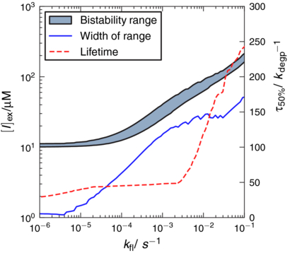
Figure 9. Dependence of the bistability range and metastable lifetime τ50% at equal induction probability on the looping rate kfl. By increasing the distance between the primary and auxiliary operators, the three-state model can be continuously changed into a two-state model. In general, faster looping rates lead to greater ranges of bistability. The minimum inducer concentration necessary for bistability also increases with the looping rate. The curves appear noisy since the fixed point n0 changes as kfl changes. See supporting information section S3 for details available at stacks.iop.org/PB/10/026002/mmedia.
Download figure:
Standard image6. Conclusions
The geometric bursting approximation coupled with FSP is a fast way to numerically solve CMEs involving transcription while accurately accounting for transcriptional noise. Formation of DNA loops in a genetic switch has a profound effect on the sensitivity of the switch to external inducer concentration, allowing it to be bistable over a much larger range of concentrations. Looping also affects the PDFs of protein copy number, allowing for fast switching times between metastable states while maintaining sharply differentiated states of induction, hinting at a possible design methodology in synthetic biology where fast, highly resolved switch states are needed.
Acknowledgments
TME would like to thank Brian Munsky for valuable discussions regarding the finite state projection during the Sixth q-bio Summer School at Los Alamos, NM. This work was supported in part by National Science Foundation through the programs Center of Physics of Living Cells (PHY-082613), the Physics of Living Systems (PHY-1026665), and DMR-1005209 and in part by the DOE Office of Science (BER) under contract number DE-FG02-10ER6510.