
Abstract
The five-dimensional generator coordinate method with the five generator coordinates being the components of the quadrupole tensor is used to generate the nuclear collective quadrupole excitations by the vibrations and rotations of the intrinsic deformed ground state of the mean-field Hamiltonian. The Gaussian overlap approximation leads to a differential eigenvalue equation with the five-dimensional Bohr Hamiltonian. The resulting collective Hamiltonian is presented. It can be calculated only approximately. However, there is a clear algorithm how to improve the approximation. Formulae for the inverse vibrational inertial functions, the moments of inertia and the potential with the vibrational and rotational zero-point energy corrections are given in the lowest-order approximation.
Export citation and abstract BibTeX RIS
1. Introduction
In spite of the long history of the Bohr Hamiltonian dating back to the 1950s [1], it remains one of the most effective tools to describe the lowest collective quadrupole excitations of the even–even nuclei (see [2]). In its general form the Bohr Hamiltonian is adapted to the description of the whole gamut of the quadrupole excitations in the nuclei with different stable and unstable deformations. However, the assumption that the quadrupole motion is adiabatic is in the nature of the Bohr Hamiltonian meaning that there is no coupling with other degrees of freedom.
Usual derivations of the Bohr Hamiltonian from the microscopic many-body theories of nuclei are based on methods of the type of the time-dependent Hartree–Fock (TDHF) method and produce classical Hamiltonians which should be requantized afterwards [3]. This is an essential reservation about such procedures. A purely quantum derivation of the Bohr Hamiltonian comes from the generator coordinate method (GCM) [4–6]. The Bohr Hamiltonian acts in the five-dimensional space of the quadrupole variables and thus five generator coordinates are required in the procedure. Although the multi-dimensional GCM was considered for a long time [7–10], it seems that the full five-dimensional Bohr Hamiltonian coming from the GCM was derived explicitly only recently [11]. This paper discusses the resulting form of the Bohr Hamiltonian which can be used for further investigations of the quadrupole excitations. In section 2 the GCM for the quadrupole collective excitations is formulated and discussed. The Gaussian overlap approximation (GOA), which leads to the Bohr Hamiltonian, is applied to the Hill–Wheeler equation in section 3. The Bohr Hamiltonian itself is discussed in section 4. Formulae needed to construct the Bohr Hamiltonian when knowing the deformation-dependent intrinsic state are given in the appendix.
2. The generator coordinate method for the quadrupole collective excitations
The GCM is a fully quantum mechanical method appropriate for the description of various collective phenomena. This is because of the concept of the generator coordinates. The choice of such coordinates determines the kind of collective motion. A relationship between the GCM and the boson expansion methods [6] suggests the point that the considered collective motion does not need to be adiabatic and a static interaction with other degrees of freedom can be taken into account.
Let the considered nucleus be described microscopically by the many-body Hamiltonian  which is invariant under the OT
(3) group of transformations, i.e. the superposition of time reversal
which is invariant under the OT
(3) group of transformations, i.e. the superposition of time reversal  and the orthogonal transformations (the rotations
  and the space inversion
  ) in the physical three-dimensional space. In order to describe its quadrupole collective excitations by means of the GCM, we should choose a suitable generating state which depends on the generator coordinates representing the quadrupole degrees of freedom. We start with an intrinsic state |ϕ(d)〉 being the ground state of the mean-field Hamiltonian of the nucleus with a given deformation d = (d0,d2) defined by the two intrinsic components of the quadrupole moment. State |ϕ(d)〉, which has the broken rotational symmetry, is assumed to be normalized to unity for every d, and even under time reversal
  , parity
  and the three signatures with respect to the intrinsic axes. The assumed symmetries tell us that it is the state of an even–even nucleus. The set of the deformation-dependent intrinsic states turned out to an arbitrary orientation with respect to the laboratory frame, namely

where ω = (ω1,ω2,ω3) are the three Euler angles of the orientation, are supposed to play the role of the GCM generating states for the quadrupole collective motion. Then, the trial state is taken in the form

where dΩ(d) = |d2(3d20 − d22)|dd0 dd2 and dΩ(ω) = sin ω2 dω1 dω2 dω3. The variational principle leads to the Hill–Wheeler integral (non-orthogonal) eigenvalue equation of the form
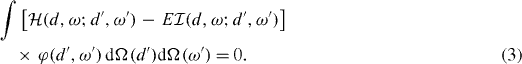
The equation is determined by the two real symmetric kernels: the overlap kernel  and the energy kernel
  . There are some technical and essential problems with solving the above equation detected when using the angular momentum projection procedure [6, 12, 13]. First of all, equation (3) contains the tedious five-dimensional integration. In addition, three-fold integration is done with respect to the periodic angle variables having a complicated topology (see [14]). This is perhaps one of the reasons why the rotational part of the Bohr Hamiltonian could hardly be derived.
To get rid of the angle coordinates, we introduce five new variables being the five components, αμ, μ = −2,...,+2, of the quadrupole tensor α = α(d,ω) defined by the relation

as the generator coordinates. The semi-Cartesian Wigner functions Dμ0 and Dμ2 are combinations of the usual Wigner functions  [11]. Real combinations ak (k = 0, 2, x, y, z) of components αμ form a vector in the five-dimensional Euclidean space. Thus, the volume element in the space of the quadrupole coordinates is

Transformation d, ω → α is reversible in the ranges 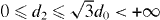 , and 0 ⩽ ω1 < 2π, 0 ⩽ ω2 ⩽ π, 0 ⩽ ω3 < 2π of variables d, ω. The generating state |Φ(d,ω)〉 = |Φ(α)〉 can thus be treated as a function of α. Finally, the trial state in the GCM is taken in the form

and the Hill–Wheeler equation reads

Another problem with equation (7) consists in the fact that the overlap kernel as a matrix with indices α and α' need not be positive definite. This problem is usually overcome by restricting the solution to the so-called collective subspace spanned by the eigenstates of the overlap with the positive eigenvalues [13]. Finally, it is possible that the overlap kernel is equal to zero at some point (some orientation). Then, a singularity can occur in the energy kernel when it is calculated within the density functional approach [15]. This causes a serious problem in solving equation (7). A similar problem occurs at the projection onto a good particle number [16, 17]. This is beyond the scope of the present paper. However, we can suspect analogies.
3. The Gaussian overlap approximation
In order to get rid of the troublesome singularities in equation (7) mentioned in the previous section, we use the GOA for the overlap kernel approximating it by the Gaussian function which is positive everywhere and has no zeros in its tails, namely

where  and γμ = αμ − α'μ (the summation convention for upper and lower indices is used—see [11]) with

The matrix g is real, symmetric and positive definite. Usually, the GOA for the energy kernel means additionally the quadratic term in the quotient of kernels, namely

with
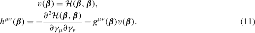
The matrix h is real and symmetric as well. Within the GOA, we overcome the difficulties mentioned in the previous section as the Gaussian overlap kernel (8) is always positive. The physical meaning of the GOA is not very clear. Because of its equivalence to the Bohr Hamiltonian model (see further below) it can be treated as the adiabatic approximation for the quadrupole collective motion.
The square root kernel
such that

where  , can be defined for the Gaussian overlap kernel (8). The integral Hill–Wheeler equation (7) in the GOA of (8) and (10) is reduced to an orthogonal eigenvalue equation for the wavefunction

It turns out that the kernel of this integral equation for ψ is a local distribution depending on the Dirac delta function and its second-order derivatives [11]. This means that the integral equation is, in fact, a differential equation. In conclusion, the Hill–Wheeler equation reduces to a differential eigenvalue equation in the GOA.
4. The Bohr Hamiltonian
The five-dimensional GCM for the quadrupole collective motion leads to the Bohr differential eigenvalue equation

with the Bohr Hamiltonian in the form

where the inverse inertial bitensor is

and the potential reads
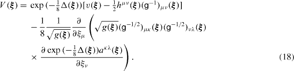
Matrices g−1 and g−1/2 are obviously such that g·g−1 = 1 and g−1/2·g−1/2 = g−1. The Laplacian is

One can say that the equivalence between the Hill–Wheeler equation (7) and the differential equation (15) in the GOA is formal only since formulae (17) and (18) for the inverse inertial bitensor and the potential, respectively, contain the exponential function of the Laplacian and, thus, the infinite number of differentiations (see [8]). However, the Bohr Hamiltonian can be determined with an arbitrary accuracy performing step by step the successive terms with the powers of the Laplacian in the corresponding power series provided that the procedure is convergent. The lowest order approximation means putting  in equations (17) and (18).
The inverse inertial bitensor of equation (17) determines the kinetic energy of the quadrupole motion which is a mixture of the vibrational and the rotational motion. In spherical nuclei the vibrations and rotations are coupled so strongly that the five-dimensional vibrations with respect to the laboratory frame are observed in the end. In deformed nuclei the quadrupole motion consists of separate rotations and vibrations. In general, a separate description of the rotational and the vibrational motion, what is often practiced so far (e.g. [18, 19]), can lead to inconsistencies. In particular, there is an opinion that a double variational method with 'generator velocities' in addition to the generator coordinates should be applied to describe the rotation [20] (see also [6, 21]). The collective potential of equation (18) contains the zero-point energy corrections associated with both, the vibrational and the rotational degrees of freedom. In general, the vibrational and rotational zero-point energy correction terms are not additive and must not be calculated separately (however, see, e.g., [22–26]). Whether the Bohr Hamiltonian in the form of equation (15) describes well enough the quadrupole excitations in real nuclei, it is a question of applications to specific cases. It should be remembered that the collective model is a bridge between a microscopic many-body theory and observable quantities.
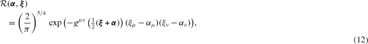
Previous schematic derivations of the Bohr Hamiltonian (see, e.g., [6, 10, 24]), which have not taken into account all the nuances of the present case of the five-dimensional quadrupole motion, have, roughly speaking, consisted of the following trick. Instead of using equation (10) the energy kernel is presented in the following form (see equation (13)):

Then, function h(α,α') is expanded in power series up to the second order for αμ and α'μ around point ξμ, which is the peak of both Gaussian functions,  and
and  , inside the integral. It is an approximation stronger than the GOA in equation (10) because it assumes in addition that h(α,α') is a slow varying function of α and α' separately. As a result, the inverse inertial bitensor and the potential in, at most, the second-order approximation of the exponential Laplace operator can be obtained in comparison with equations (17) and (18).
5. Summary
Knowing an intrinsic deformed state which is a function of the quadrupole deformation, we can generate the five-dimensional collective quadrupole excitations within the frame of the multi-dimensional GCM. It is convenient to use the five generator coordinates being the laboratory components of the quadrupole deformation tensor. In the GOA, which can be treated as the adiabatic approximation for the quadrupole collective motion, the integral Hill–Wheeler equation is equivalent formally to the eigenvalue equation for the Bohr Hamiltonian. This Hamiltonian is determined by the weight being a measure of the Gaussian overlap width, the inverse inertial quadrupole bitensor and the potential. The inverse inertial functions and the potential can be calculated only in an approximation. However, it can, in principle, be done with an arbitrary accuracy. Finally, the Bohr Hamiltonian can be calculated knowing the intrinsic state as a function of the quadrupole deformation. It is a challenging question how the GOA Bohr Hamiltonian describes the collective quadrupole states in comparison with that obtained from the TDHF methods.
Appendix.: The Bohr Hamiltonian in the intrinsic coordinates
The Hill–Wheeler equation in the GOA and thus the Bohr Hamiltonian are originally determined by quadrupole scalar v(α) and the two symmetric matrices, g(α) and h(α), being quadrupole symmetric bitensors. Below we compile the formulae needed to calculate them and other quantities appearing in the Bohr Hamiltonian. According to equations (9) and (11) v, g and h are expressed by kernels  and
and  and their derivatives of the second order with respect to the quadrupole variables αμ. The relation between the derivatives with respect to αμ and the derivatives with respect to the Euler angles and the intrinsic components d0, d2 reads [2]
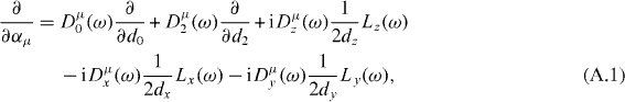
where

and the intrinsic components of the drift angular momentum of the rotation of the intrinsic frame, Lx(ω), Ly(ω), Lz(ω) are differential operators with respect to the Euler angles [2] and fulfill the relation 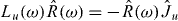 for u = x,y,z (
 are the intrinsic components of the many-body total angular momentum). Using (1) and (A.1) v, g and h can be expressed by the overlaps of the intrinsic states and/or their derivatives with respect to the deformations, and matrix elements of operators
  ,
,  ,
,  and
and  in the basis of the intrinsic states which possess the time reversal, parity and signature symmetries mentioned in section 2. For v, we have obviously

The matrix g can be presented in the following form:

where a, b = 0, 2, x, y, z, and the matrix of the intrinsic Cartesian components gab(d) reads


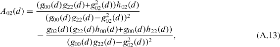
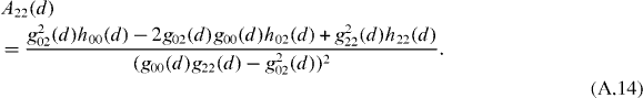
where |ϕk(d)〉 = ∂|ϕ(d)〉/∂dk, etc. Its determinant is g(d) = g2v(d)gxx(d)gyy(d)gzz(d) and g2v(d) = g00(d)g22(d) − g202(d). It is worth noting that every symmetric matrix, which is an isotropic function of a quadrupole tensor, is determined by six intrinsic Cartesian components and has the structure given by (A.4) and (A.7) (see [2]). Thus, it is sufficient to give the six non-vanishing intrinsic Cartesian components of matrices g−1 and g−1/2 which are also in the game. They read
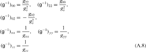
and
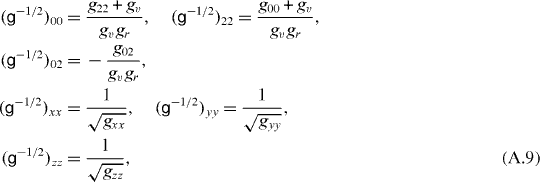
where 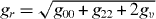 . The intrinsic Cartesian components of the matrix h are equal to
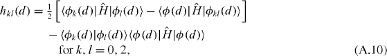
Here we take the lowest order approximation putting 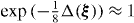 in equations (17) and (18). The six intrinsic Cartesian components of the inverse inertial bitensor are usually called the inverse inertial functions, the vibrational and the rotational ones. The vibrational inverse inertial functions are equal to

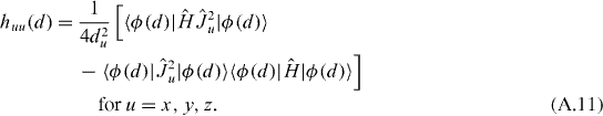
All of them depend only on the vibrational (with indexes 0 and/or 2) intrinsic Cartesian components of matrices g and h. The rotational inverse inertial functions are equal to

for u = x, y, z. They depend in turn only on the rotational intrinsic Cartesian components of matrices g and h, which are functions of matrix elements of operators  ,
,  ,
,  and
and  and do not contain the derivatives of intrinsic states with respect to the deformations. The moments of inertia by definition (see [2]) are
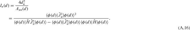
They resemble the Yoccoz moment of inertia [27] and have a form similar to those of a rigid body [28].