


Abstract
This study theoretically and experimentally investigates the phase structure of radiation emitted from an elliptically polarized undulator. Analytic expressions for the emitted electromagnetic fields are fully derived and the radiation's phase structure is found to change according to polarization. When the polarization is circular, a helical structure is observed; however, when the polarization changes from circular to elliptical, a phase structure comprising several orbital angular momentum modes is observed. Herein, phase gradients of the undulator's radiation are measured using a double-slit interferometer. A sampling moiré method is used to accurately extract the phase difference on the transverse plane from the observed interference fringe. The measured phase gradients of the first and second harmonics reveal a similar change to the calculated results. However, under circular polarization, the change exhibited by the third harmonic is smaller than the calculated value. This phase gradient reduction is due to the split in phase singularities and is attributed to both the fluctuation in the undulator's peak magnetic fields and the radiation emitted from the entrance and exit of those magnetic fields.
Export citation and abstract BibTeX RIS

Original content from this work may be used under the terms of the Creative Commons Attribution 4.0 licence. Any further distribution of this work must maintain attribution to the author(s) and the title of the work, journal citation and DOI.
1. Introduction
Light can carry both spin angular momentum and orbital angular momentum (OAM) [1]. The former arises from circular polarization, whereas the latter results from the phase structure of light. For over two decades, the light-forming helical phase structure known as an optical vortex has been actively studied; this includes research on the generation of these phase structures using special optical elements [2] and applications, such as quantum entanglement [3], data transmission [4], astrophysics [5], and the exploration of their interaction with atoms and materials [6–8].
Optical vortices can be spontaneously generated from a free electron without using typical special optical elements. The trajectory of the electron is instrumental in this process. Katoh et al revealed that an electron requires a circular trajectory to generate the radiation that forms a helical phase structure [9]. The required circular motion of an electron can be induced by a circularly polarized helical undulator [10–15], a circularly polarized intense laser beam [16–18], and an electron cyclotron emission [19]. Recently, the radiation emitted from a cycloid-shaped trajectory, which is a superposition of two circular trajectories, was found to possess a helical phase structure [20]. Thus, these simple radiation processes can generate an optical vortex extending from the radio to gamma-ray wavelength regions.
This study presents the first theoretical and experimental investigation on the phase structure of radiation generated from an elliptical trajectory. Although an elliptically polarized laser can be used to achieve an electron's elliptical trajectory, this research uses an elliptically polarized undulator [21–24] as there are techniques to measure the phase structure of ultraviolet light. Theoretical expressions for elliptically polarized undulator radiation are fully derived herein to calculate the phase structure of the emitted radiation. Phase structure is found to change according to polarization: specifically, when the polarization shifts from circular to elliptical, splits occur in the phase singularities in harmonics higher than the second harmonic. Furthermore, to confirm the proposed theory, this study reports on an experiment conducted at the synchrotron radiation facility, UVSOR-III [25]. The phase gradients of the undulator radiation are measured using a double-slit interferometer and a sampling moiré method. The measured phase gradients of both the first and second harmonics exhibit a similar change to the calculated results; however, the change demonstrated by the circularly polarized third harmonic is smaller than that obtained via calculation. This study demonstrates that this reduction in change originates from a distorted annular intensity distribution caused by the split in the phase singularities.
New phenomena are predicted in the dichroic effect [26], photoionization [27], and Thomson scattering [28] in optical vortices at both ultraviolet and x-ray frequencies. This article discusses a high-energy light source with a controllable phase structure, which may reveal new research opportunities in related fields of study. The production of an optical vortex with a large OAM in the x-ray region is of particular interest [29–31]. High harmonic radiation emitted from a circularly polarized undulator has the advantage of producing a large OAM as the nth harmonic radiation carries an OAM of (n − 1)ℏ, where ℏ is the Planck constant divided by 2π. A clear annular intensity distribution is a critical characteristic for an optical vortex carrying a well-defined OAM. The findings presented herein will contribute to the design of an undulator for producing a short-wavelength optical vortex carrying a large OAM.
2. Derivation of theoretical equations
2.1. Electron trajectories of an elliptically polarized undulator
Theoretical analyses for an elliptically polarized undulator have been conducted in [21–24]. Typically, the radiation energy, which is proportional to the square of the absolute value of an emitted electric field from an electron, is derived. However, a phase term, which is important when considering the phase structure, is absent in such an equation. This study derives the explicit expressions of emitted electric fields from an electron moving inside an APPLE-II-type undulator to calculate both its phase structure and its spatial intensity distribution.
Here, the electron is assumed to move along the z-direction, and the origin of the z-axis is set at the upstream edge of the undulator. The coordinate system used in the calculation is shown in the inset of figure 3. The on-axis magnetic fields of an APPLE-II-type undulator are expressed as (equations (5) and (6) in [32]):

and

where B0 is the coefficient, D is the undulator phase (see figure 1 of [32]), and ku = 2π/λu, where λu represents the period length of an undulator. The electron orbits described in the Cartesian coordinate system can be derived by solving the relativistic Lorentz equations using these magnetic fields, which are expressed as follows:
Here, Kx = K| cos(D/2)|, Ky = K| sin(D/2)|, and K = eB0/(mecku) are the deflection parameters of an undulator; e is the elementary charge; me is the electron mass; c is the speed of light; γ is the Lorentz factor of the electron; ωu = kuc⟨βz⟩,  ; sgn() is the sign function; and t represents time. The ratio of the deflection parameters, Ky/Kx, is the critical parameter for characterizing the polarization. When Ky/Kx = 1, the polarization is circular, and an electron moves on a perfect circular trajectory in the x–y plane. When 0 < Ky/Kx < 1, the polarization becomes elliptical: the transverse electron's orbit follows an elliptical trajectory. When Ky/Kx = 0, the polarization is linear along the x-axis, and an electron moves along the x-axis. Furthermore, the motion of the electron possesses helicity, which is determined by the undulator phase. When an observer faces an oncoming electron and when D < 0 (D > 0), the electron follows an elliptical trajectory in the counterclockwise (clockwise) direction; this is termed positive (negative) helicity.
2.2. Electric fields of elliptically polarized undulator radiation
The Lienard–Wiechert potentials (section 14.5 in [33]) can be used to calculate the Fourier component of the electric field emitted by a single electron in an arbitrary orbit and normalized velocity, as follows:

where k = ω/c and ω are the wave number and angular frequency of the emitted radiation,  0 is the permittivity of the vacuum, R is the distance from the origin to the observation point, n is a unit vector pointing from the origin to the observation point, and β is the velocity vector of the electron. Equation (4) is calculated in the spherical coordinate system (r, θ, ϕ) and unit vectors (er, eθ, eϕ) with the application of the following relations: n × (n × β) = −(β ⋅ eθ)eθ − (β ⋅ eϕ)eϕ. In the spherical coordinate system, each electric field component can be expressed as follows:
and
Here, N is the number of the period of an undulator magnetic field; Jn+μ = Jn+μ−2s(b1)Js(b2) exp(iμξ) (μ = 0, ±1, and ± 2);  ;
;  ; n and s are the integers; Jn() is the Bessel function of the first kind;
  , and
, and

when θ ≪ 1. Equations (5) and (6) are sharply peaked at the angular frequency given by ω = nω1. The energy of the nth harmonic radiation can thus be described as

The energy of the undulator radiation is maximized at the central axis (θ = 0) and decreases with θ.
The electric fields are expressed by the complex orthogonal unit vectors,  ; their circular polarization helicities are positive and negative, respectively, to demonstrate the phase structure in the transverse plane. Here, the unit vectors along the x- and y-axes are represented by ex and ey, respectively. The electric field will be [16]

where

and

The z component in the paraxial approximation (θ ≪ 1) is ignored.
3. Numerical calculation of spatial distribution, phase distribution, and orbital angular momentum distribution under a general condition
Radiation energy per unit of angular frequency and unit of solid angle is expressed as (section 14.5 in [33]):

where dΩ = dϕ dθ sin θ. Figures 1 and 2 contain both the calculated radiation energies for E+ and E− and the phase distribution determined by  . Here, the helicity of the electron's motion is shown to be positive, implying D < 0. The calculation parameters are λu = 88 mm, N = 10 in both figures, γ = 900, K = 4.19, and n = 2 in figure 1 and γ = 784, K = 4.50, and n = 3 in figure 2. These parameters correspond with the experimental condition. The wavelength of emitted radiation at the center axis (θ = 0) calculated using equation (8) is 266 nm and it is the same for all polarization states as equation (8) is a function of
  , which is independent of Ky/Kx.

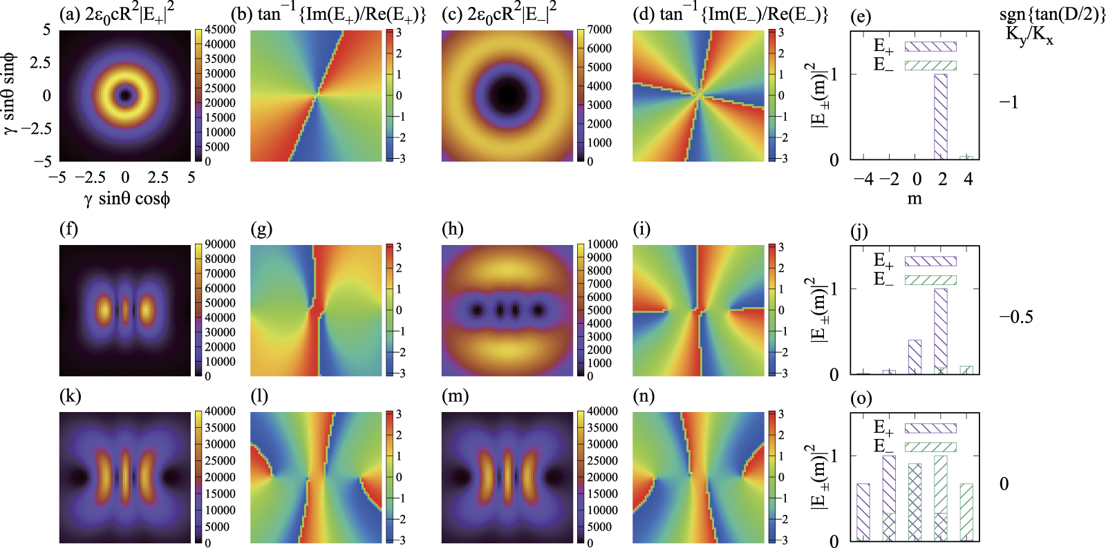
Figure 1. (a), (c), (f), (h), (k) and (m): calculated spatial distribution of the second harmonic (n = 2) radiation energy per unit of angular frequency and the solid angle for E+ and E−. (b), (d), (g), (i), (l) and (n): phase distribution for E+ and E−. (e), (j) and (o): distribution of OAM at a polar angle of θ = 2/γ. The parameter  are (a)–(e): −1, (f)–(j): −0.5 and (k)–(o): 0, as indicated in the panels. The calculation parameters are γ = 900, K = 4.19, λu = 88 mm, ω = nω1, and N = 10, which correspond with the experimental condition.
Download figure:
Standard image High-resolution image
Figure 2. The same as figure 1, except for the third harmonic (n = 3), γ = 784, and K = 4.50.
Download figure:
Standard image High-resolution imageWhen the electron's trajectory is circular ( ), the positive and negative helicity components of the emitted radiation possess the phase terms of exp {i(n − 1)ϕ} and exp {i(n + 1)ϕ}, respectively. Therefore, the phase possesses periodic natures of 2π(n − 1) for positive helicity and 2π(n + 1) for negative helicity, as shown in figures 1(b) and (d) and 2(b) and (d), respectively. Owing to the phase singularities at the central axis, the annular intensity distribution is clearly observed in figures 1(a) and (c) and 2(a) and (c). In the actual experiment, the positive helicity component is primarily observed, as it is far stronger than the negative component. These results are consistent with those of previous works [9, 10, 16, 34].
Under an elliptical electron trajectory ( ), a phase structure is clearly observed in the emitted radiation, which is distorted by circular polarization (figures 1(g) and 2(g)). Moreover, in the negative helicity of the second harmonic and in both helicities of the third harmonic, the phase singularity is split one by one; this is evident in figures 1(i) and 2(g) and (i). These split-phase singularities ultimately settle between the bright linear polarization (Ky/Kx = 0) peaks, as presented in figures 1(k)–(n) and 2(k)–(n). It is widely accepted that the nth high harmonic radiation of the linear polarization has n intensity peaks along the direction of polarization [35]; these features can be explained by electron motion [36]. Notably, the dark spots between the peaks are phase singularities; this provides an intuitive understanding of the intensity distribution of linearly polarized undulator radiation. Furthermore, the uniformity of the total phase distribution of the linear polarization is noted as it is a superposition of the circular polarization with both positive and negative helicities, which are symmetric to each other.
The OAM and azimuthal angular position are related by a Fourier transform [37–39]. The distribution of the discrete values of the OAM, mℏ, can be calculated using the method presented in [39]:

|E±(m)|2 is presented in figures 1(e), (j) and (o) and 2(e), (j) and (o). As shown in figures 1(e) and 2(e), when the polarization is circular, OAM has only one component at m = n − 1 for positive helicity and at m = n + 1 for negative helicity; however, in the elliptical polarization illustrated in figures 1(j) and 2(j), other OAM components appear. Therefore, different average OAM values are carried by the elliptically polarized radiation compared with circular polarization. Multiple OAM components are evident in the linear polarization (figures 1(o) and 2(o)); however, the average OAM becomes zero because the OAM distribution is symmetric with respect to m = 0.
4. Measurement and calculation results of the phase gradient
An interference fringe measurement between a reference wave and an optical vortex wave is a commonly used approach used to assess the phase distribution and OAM [39]. To apply this method to undulator radiation, tandem undulators are required, as reported in previous studies [11, 13]. However, this approach convolutes the characteristics of dual undulator radiation. Therefore, to examine the phase structure of single undulator radiation, measuring an interference fringe from a double slit is necessary. Interference fringes from a double slit of the first and circularly polarized second harmonics were measured in [13]. It was observed that the interference fringes were explicitly distorted around the phase singularity. In this study, the interference fringes of the first through third harmonics in various polarization states are measured while scanning a double slit to measure an average phase gradient.
Undulator radiation possesses a broad spectrum. To measure a clear interference fringe, a complementary metal oxide semiconductor (CMOS) camera (Bitran, CS-66UV) was used to detect the undulator radiation passing through two bandpass filters (BPFs) (Semrock, LL01-266-25 and Edmund Optics Inc., #67-878). The center wavelength and the total bandwidth of the two BPFs were 265.9 nm and 1.9 nm in full width at half maximum, respectively. The total transmittance was 8% at 265.9 nm and less than 0.01% in the other wavelength range. Two BPFs were attached in front of the CMOS camera, and the pixel size and pixel format of the camera were 6.5 μm and 2048 × 2048, respectively.
4.1. Electron beam and APPLE-II-type undulator
The experiment was conducted at the BL1U beamline of the synchrotron radiation facility, UVSOR-III [12, 13, 15]. For such an interference experiment using a double slit, the transverse coherence of the undulator radiation is essential. Consequently, an electron beam was operated at the energies of 400 MeV (γ = 784) and 460 MeV (γ = 900), which are lower than the typical electron beam energy of 750 MeV, to reduce the emittance of the electron beam to 5.0 and 6.6 nm-rad, respectively. In the ultraviolet wavelength range, the radiation emitted from such a diffraction-limited electron beam is transversely coherent. During the experiment, the typical electron beam current was less than 1 mA.
An APPLE-II-type undulator was located at the BL1U. The undulator's period length, λu, and the number of periods of magnetic fields, N, were 88 mm and 10, respectively. The magnet rows were mechanically moved to adjust both the polarization and wavelength of the undulator radiation [32]. A gap and a phase of the magnet rows were adjusted so that the wavelength of undulator radiation, which was measured with a spectrometer, corresponds with 266 nm. To enable the use of ordinary optical components and devices, undulator radiation was extracted from the vacuum via a quartz window in the atmosphere. Notably, the undulator radiation was directly extracted without passing through any optical components such as mirrors or monochromators, which might influence the phase structure. The distance between the center of the undulator and the quartz window was 7150 mm. The CMOS camera was located 250 mm away from the quartz window and was used to measure the intensity distribution of the undulator radiation. Therefore, considering the size of the sensor, the radiation was measured in the range of θ < 0.90 mrad, which is narrower than the range of θ < 5.6 mrad and θ < 6.4 mrad presented in figures 1 and 2, respectively. In this study, undulator radiation was measured only around the central axis.
4.2. Phase gradient
4.2.1. Measurement of interference fringes from a double slit
Figure 3 presents a schematic of the experiment. The double slit and the CMOS camera were located at distances of 150 and 1240 mm, respectively, from the quartz window. The double slit comprised two rectangular slits with a dimension of 0.1 × 20 mm; the 20 mm longitudinal length was sufficiently larger in size than the detection area of the CMOS camera, and there was a distance of 1 mm between the centers of the two slits. The double slit was patterned on a quartz substrate at a thickness of 0.7 mm via ultraviolet lithography. To ensure backward reflection of the incident beam, the non-transmission area was masked by spattered chromium. The double slit was mounted on a triple-axis stage, which included two linear stages and a rotation stage. The double slit was scanned a total of seven times in increments of 1 mm along the x-direction before rotating through 90° and scanning along the y-direction. The rotation angles of the double slit along the x- and y-directions were adjusted so that the interference fringe of the first harmonic becomes parallel against the coordinate system of the CMOS camera. The accuracy of this method is estimated as 0.6 mrad.

Figure 3. Schematic of interference fringe measurement using a double slit.
Download figure:
Standard image High-resolution image4.2.2. One-dimensional phase difference analysis using a sampling moiré method
An interference fringe from a double slit can be expressed as [40, 41]

where A and B are the background and amplitude intensities of the interference fringe; P = λL/a is the fringe pitch; and φ is the phase value of the interference fringe. Additionally, a is the distance between the centers of the two slits (1 mm); λ is the observed wavelength of the undulator radiation (265.9 nm); L is the distance between the double slit and the CMOS camera (1090 mm); and ΔΦ is the phase difference of the undulator radiation passing through the individual slits. When ΔΦ is a constant value, the interference fringe exhibits a periodic straight pattern; however, the pattern is distorted if ΔΦ is not constant along the longitudinal direction of the slit, as observed in figure 1 in reference [42].
Various methods of phase analysis can be applied to extract ΔΦ from a single interference fringe, such as Fourier transform [43, 44], wavelet transform [45], and windowed Fourier transform [46]. To analyze both the phase and phase gradient distributions of the interference fringe, this study utilized a sampling moiré method [47] as a fast and accurate spatial phase analysis technique for a single fringe pattern [48].
According to the theory of the sampling moiré method [49], after applying down-sampling with a sampling pitch and intensity interpolation for the recorded interference fringe to obtain multiple phase-shifted moiré fringes, three unknown parameters of A, B, and φ can be simultaneously determined using the discrete Fourier transform algorithm.
The calculation of a normalized interference fringe with a constant amplitude facilitated the clear visualization of the change in phase difference. The normalized fringe pattern, Ĩ, was obtained by substituting the background and amplitude intensities to the original interference fringe, as expressed in equation (15). Reference [50] contains the detailed procedure of the normalization calculation.

In this experiment, a 15-pixel (97.5 μm) sampling pitch was used to calculate the phase and phase difference distributions via the sampling moiré method. A one-dimensional phase difference distribution along the center line of a double slit was extracted from a normalized interference fringe.
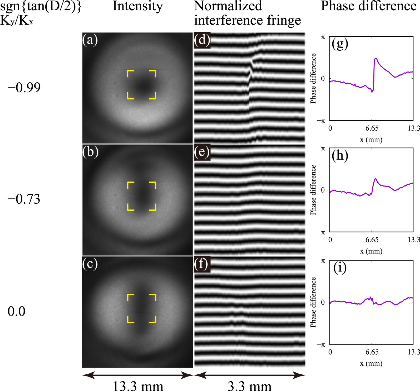
Figures 4 and 5 show examples of measured intensity distributions, the normalized interference fringes, and the one-dimensional phase difference distributions for the second and third harmonics, respectively. In the second harmonic, a clear annular shape is observed in the spatial distribution of the circularly polarized radiation; the intensity is higher along the horizontal direction than in the vertical direction as the polarization changes to linear from circular, as shown in figures 4(a)–(c). This is consistent with the calculation presented in figure 1. As discussed in section 3, a phase of circularly and elliptically polarized radiation changes around a phase singularity. Figures 4(d) and (e) illustrates that the interference fringe along the horizontal direction is explicitly distorted in the circular polarization and is slightly distorted in the elliptical polarization around the phase singularity. Consequently, a change in phase difference around the phase singularity occurs, as observed in figures 4(g) and (h). Figures 4(f) and (i) reveals that in linear polarization, because a phase is uniform in the transverse plane, both the interference fringe and phase difference are almost constant along the horizontal direction.
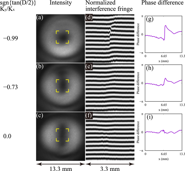
Figure 4. (a)–(c): measured intensity distributions of the second harmonic. (d)–(f): normalized interference fringes in the region of the dashed yellow boxes indicated in (a)–(c) when the slit is aligned along the x-direction. (g)–(i): one-dimensional phase difference distributions along the horizontal center line of the dashed yellow boxes. The parameter,  , is (a), (d) and (g): −0.99, (b), (e) and (h): −0.73 and (c), (f) and (i): 0.0, as indicated in the panels. The energy of the electron beam is 460 MeV.
Download figure:
Standard image High-resolution image
Figure 5. (a)–(c): measured intensity distributions of the third harmonic. (d)–(h): normalized interference fringes in the region of the dashed yellow boxes indicated in (a)–(c) when the slit is aligned along the x-direction. (i)–(k): one-dimensional phase difference distributions along the horizontal center line of the dashed yellow boxes. The parameter,  , is (a), (d), (e) and (i): +1.0, (b), (f), (g) and (j): +0.88 and (c), (h) and (k): 0.0, as indicated in the panels. The energy of the electron beam is 400 MeV.
Download figure:
Standard image High-resolution imageThe calculation for the third harmonic confirms that there are two phase singularities; their separation is amplified as the circular polarization changes to elliptical, as figure 2 illustrates. Two phase singularities (two dark spots) are observed in both the circular and elliptical polarizations; furthermore, as figures 5(a), (b) and (d)–(g) shows, there is explicit distortion of the interference fringes around these phase singularities. In the elliptical polarization and as observed in figures 5(b), (f), (g) and (i), two phase singularities along the horizontal direction are aligned. This result agrees well with the calculation presented in figure 2(g). However, the difference in intensity distribution between figures 2(f) and 5(b) is due to the different Ky/Kx and observation region. In the circularly polarized third harmonic, no clear annular shape can be detected; this is discussed in section 5. Similar to the case of the second harmonic, both the interference fringe and phase difference of the linear polarization are almost constant along the horizontal direction, as can be observed in figures 5(h) and (k).
4.2.3. Two-dimensional phase analysis
The phase gradient around the center of the beam can be obtained by measuring the phase difference distribution in two dimensions and applying the following equation:

Here, ΔΦy and ΔΦx are the phase differences for the slit aligning along the x- and y-axes, respectively; these are extracted from the interference fringes, as described above. Figures 4(g)–(i) and 5(i)–(k) present examples of ΔΦy. The phase gradient is averaged within a square of 6.5 × 6.5 mm2 around the central axis for the first and second harmonics and a square of 9.3 × 9.3 mm2 around the central axis for the third harmonic, when |ΔΦx,y| < π is satisfied.
For a comparison between the measurement and the calculation, the determined phase gradient based on equations (10) and (11) is defined, as follows:

Here,  . The phase gradient is averaged within a square of 13.3 × 13.3 mm2, which corresponds with the detection area of the CMOS camera when the intensity at each position in the x–y plane is greater than 5% of the maximum intensity. Additionally, this threshold corresponds to the noise level of a CMOS camera. Furthermore, the distance between an undulator and a plane at the location of the phase gradient calculation also corresponds with the experimental condition. The phase gradient calculated using equation (17) is represented by solid lines in figures 6(a)–(c) along with the measured phase gradient determined by equation (16), which is indicated for each harmonic by circular, square, and triangular marks.
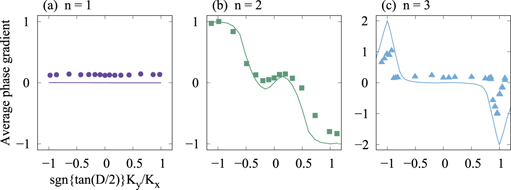
Figure 6. (a)–(c): calculated and measured average phase gradients for (a): the first, (b): the second, and (c): the third harmonics. Solid lines represent the calculated results. The circular, square, and triangular marks represent the measured results for the first, second, and third harmonics, respectively. The uncertainty of the measured value is less than the size of the symbols. The electron beam energy is (a) and (b): 460 MeV and (c): 400 MeV.
Download figure:
Standard image High-resolution imageThe calculated phase gradient of the first harmonic is always zero, as observed in figure 6(a); this is because the radiation is a plane wave in the paraxial approximation, and it does not possess a phase structure. The measured phase gradient shows constant values as Ky/Kx varies, which is consistent with the calculation. However, the measured phase gradient adopts a non-zero value because the double slit along the horizontal direction is inclined approximately 0.35 mrad against the coordinate system of the CMOS camera.
Figure 6(b) shows that the calculated phase gradient in the second harmonic adopts ±1 for the circular polarization because there is a phase variation of 2π along the azimuthal angle (see figure 1(b)). Additionally, the phase gradient adopts values between ±1 for the elliptical polarization and zero for the linear polarization. As one phase singularity of the second harmonic is always located at the central axis, even when the polarization shifts, the phase gradient continuously changes against Ky/Kx, as observed in figures 1(b), (g) and (l). Similar changes are demonstrated by both the measured phase gradient and the calculation.
In the third harmonic represented in figure 6(c), the calculated result for the circular polarization reveals a phase gradient of ±2 as the phase varies by 4π (figure 2(b)). As the polarization state changes from circular to elliptical, the calculated value rapidly decreases; it adopts zero in most elliptical polarization states, including linear polarization. This is due to the splitting of two phase singularities from the central axis, which locates them outside the observation region when the polarization switches from circular to elliptical. A qualitatively similar trend is observed by the measured average phase gradient, although under circular polarization, the measured value is smaller than the calculated one. The cause of this is discussed in section 5.
5. Discussion
As reported in sections 4.2.2 and 4.2.3, a clear annular shape was observed in the second harmonic and the measured phase gradient demonstrated a similar change to the calculation. However, in the third harmonic, no clear annular shape was observed, and the measured phase gradient was smaller than the calculation. These two phenomena are closely related. The positions of the two phase singularities of the third harmonic are presented in figure 7(a). Ideally, under circular polarization, these two singularities are located at the central axis, and they are split along the horizontal (vertical) direction when Ky/Kx < 1.0 (Ky/Kx > 1.0). However, as the two measured phase singularities are not located at the central axis in all polarization states, a clear annular shape was not observed. As figure 7(b) demonstrates, the average phase gradient depends on the positions of the phase singularities from the central axis. When two phase singularities are located at the center, a phase induces variations in entire regions in the transverse plane, producing an average phase gradient of −2. Conversely, when two phase singularities are split and a non-zero intensity appears at the central axis, a phase is constant around the central axis, as observed in figures 2(f) and (g). Consequently, the average phase gradient is reduced.

Figure 7. (a) Positions of two phase singularities of the third harmonic, which changes with Ky/Kx. The dashed line represents the calculation, and the dots are the measurements. The color indicates the individual phase singularities. The values of Ky/Kx are indicated in the panel. (b) Average phase gradient as a function of the distance  of the phase singularities from the central axis. The solid line represents the calculation, and the dots are the measurement results. The radius of the measured data is an average value of the two phase singularities.
Download figure:
Standard image High-resolution image
The authors consider that the split in phase singularities is derived from the fluctuation of peak magnetic fields of the undulator and the radiation emitted from the entrance and exit of the undulator's magnetic fields [51]. The magnetic field measurement for the undulator used in this experiment revealed that a maximum fluctuation of 5% occurred in Ky/Kx for each magnetic period. The theoretical calculation shows that two phase singularities move to a position with a radius of 3 mm, and the phase gradient is reduced by 18% when Ky/Kx is reduced by 6% from unity, which may result in a split in phase singularities. Additionally, this study investigated an effect of the radiation emitted from the entrance and exit of undulator magnetic fields using the simulation code Synchrotron Radiation Workshop [34] because such radiation was not considered in the derived theoretical equations. Furthermore, this research discovered that radiation also affects the split in phase singularities. However, more study is required to quantitatively explain the findings.
6. Conclusion
This study demonstrated that elliptically polarized undulator radiation produces variations in phase structure. It was revealed for the first time that a change in polarization from circular to elliptical causes the phase singularities of the third harmonic to split. The measured phase gradients of the first and the second harmonics exhibited a similar change to the calculated results; however, the change in the circularly polarized third harmonic was smaller than that calculation owing to the distorted annular intensity distribution caused by the split in phase singularities. A clear annular intensity distribution is an important characteristic for an optical vortex carrying a well-defined OAM. Therefore, to generate short-wavelength optical vortices with an annular intensity distribution, the design of an undulator must consider the fluctuation in peak magnetic fields and the radiation emitted from the entrances and exits of an undulator's magnetic fields. In future work, the authors will develop a technique for measuring the OAM of undulator radiation in addition to the phase gradient reported herein.
Acknowledgments
This work was supported by a Grants-in-Aid for Scientific Research (KAKENHI) from the Japan Society for the Promotion of Science (Grant 18H03477) and the NINS program for cross-disciplinary study (Grant 01311802). Yoshitaka Taira (YT) would like to thank Dr. Katsuya Oguri at NTT Basic Research Laboratories for inspiring him to start this research. YT would also like to thank Dr. Hirokazu Kobayashi at Kochi University of Technology for the discussion on OAM measurement. The authors also thank the Equipment Development Center at the Institute for Molecular Science for fabricating a double slit.