


Abstract
The slime mold Dictyostelium discoideum is a well known model system for the study of biological pattern formation. In the natural environment, aggregating populations of starving Dictyostelium discoideum cells may experience fluid flows that can profoundly change the underlying wave generation process. Here we study the effect of advection on the pattern formation in a colony of homogeneously distributed Dictyostelium discoideum cells described by the standard Martiel–Goldbeter model. The external flow advects the signaling molecule cyclic adenosine monophosphate (cAMP) downstream, while the chemotactic cells attached to the solid substrate are not transported with the flow. The evolution of small perturbations in cAMP concentrations is studied analytically in the linear regime and by corresponding numerical simulations. We show that flow can significantly influence the dynamics of the system and lead to a flow-driven instability that initiate downstream traveling cAMP waves. We also show that boundary conditions have a significant effect on the observed patterns and can lead to a new kind of instability.
Export citation and abstract BibTeX RIS
1. Introduction
In reaction–diffusion systems, an advective flow can induce unique emergent phenomena. One well known example is the differential flow induced chemical instability (DIFICI) that destabilizes an otherwise spatially homogeneous state of a system. DIFICI was originally predicted by Rovinsky and Menzinger [1, 2] and later confirmed experimentally for the Belousov–Zhabotinsky reaction [3, 4]. The basic idea behind DIFICI is that the reacting species flow at different speeds. This differential transport can initiate instabilities of the homogeneous steady state that induce propagating wave trains moving in the flow direction. Later, conditions for the emergence of three-dimensional spatial and spatiotemporal patterns due to DIFICI were derived by Malchow [5, 6] and demonstrated by patterns in a minimal phytoplankton–zooplankton model [7]. Instabilities in the homogeneous distribution can arise if phytoplankton and zooplankton move with different velocities, regardless of which one is faster. This mechanism of generating spatial structures is free from the restrictions of the Turing mechanism [8], which requires a large difference in diffusion coefficients of the two species involved. Accordingly one can expect DIFICI to be found widely in population dynamics [9] and biological morphogenesis [10].
Recently we conducted experiments to study the effect of a differential flow in a biological system, namely quasi one-dimensional colonies of the signaling amoebae Dictyostelium discoideum (D. d.) [11]. The aggregation of D. d. amoebae after nutrient deprivation is one of the best model systems for the study of spatial–temporal pattern formation at the multicellular level. Starved D.d. cells aggregate to form a multicellular structure by directional movement of cells in response to concentration changes of the chemoattractant cyclic adenosine monophosphate (cAMP) [12–14]. D. d. cells can be excitable [15, 16], and when stimulated with extracellular cAMP, they produce more cAMP, which in turn stimulates neighboring cells [17, 18]. This excitable response explains the wavelike pattern of cAMP, which propagates in the form of either concentric or spiral waves from the self-organized aggregation centers. In the natural environment, this aggregation occurs in forest soil and can be subject to water flow. In general, this medium into which the cAMP is released is a moving fluid while the cells are crawling on a solid substrate and are not transported by the flow.
In our recent experiments with chemotactically active populations of D.d. cells [11], a narrow straight microfluidic channel was used and cells were allowed to settle on the glass substrate before a laminar flow of buffer solution through the channel was started. This flow was not strong enough to detach the cells from the substrate and extracellular cAMP molecules were advected downstream. This differential transport in the extracellular medium induced macroscopic wave trains that developed spontaneously, propagated in the flow direction and had a unique period.
In this work, we have investigated the mechanisms of flow-driven waves using the well-established two and three component Martiel–Goldbeter (MG) model [19]. In the linear regime, our analytical calculations show that the convective transport of extracellular cAMP in a uniform field of signal-relaying cells leads to a flow-induced instability of the traveling-wave type. In the nonlinear regime, numerical simulations show propagating waves initiated by a convective instability, in agreement with the predictions of the linear analysis.
2. The MG model
The kinetics of the cAMP production in well-stirred suspensions of D. d. cells are well described by the MG model [19], which is based on the relevant kinetic rate laws and the interaction between cAMP and its membrane receptor (see figure 1). In this model, extracellular cAMP binds to the receptor, and the receptor-cAMP complex activates adenylate cyclase which is an enzyme that produces intracellular cAMP from ATP. The newly synthesized cAMP is excreted into the extracellular medium where it binds to active receptors on the membrane and provides a feedback loop. A constant build up and accumulation of cAMP in the extracellular medium is limited by desensitization of the cAMP receptor upon prolonged exposure to high concentrations of cAMP. The receptor converts to an inactive form and loses its capacity to stimulate adenylate cyclase and synthesize more cAMP. Meanwhile extracellular phosphodiesterase which is supplied by the cells at a steady rate [20] degrades the cAMP in the system and in the absence of cAMP, the receptors slowly recover back to the active form. Note that the MG model is a mean-field type approximation and stochastic fluctuations are essentially neglected. The dynamics of the signaling system is given by the following set of coupled nonlinear ordinary differential equations


with
where t is equal to the real time multiplicated by k1, ρ is the fraction of receptors in the active state,  =
= ![${{[{\rm cAMP}]}_{{\rm intracellular}}}/{{K}_{R}}$](https://content.cld.iop.org/journals/1367-2630/17/6/063007/revision1/njp514795ieqn2.gif) and
and 
![${{[{\rm cAMP}]}_{{\rm extracellular}}}/{{K}_{R}}$](https://content.cld.iop.org/journals/1367-2630/17/6/063007/revision1/njp514795ieqn4.gif) are dimensionless concentrations of intracellular and extracellular cAMP, respectively. Here
are dimensionless concentrations of intracellular and extracellular cAMP, respectively. Here  is the dissociation constant of cAMP-receptor complex in an active state and
  is the desensitization rate of active receptors. The dimensionless parameters are
  ,
,  ,
,  ,
,  ,
,  ,
,  ,
,  ,
,  ,
,  and
and  . The values of model parameters are
  ,
,  ,
,  ,
,  ,
,  ,
,  ,
,  ,
,  ,
,  ,
,  ,
,  ,
,  ,
, 
 . These parameter values are the experimental data listed in the last column of table II in [17], except for the values of k1 = 0.09 min−1 and k2 = 1.665 min−1 which are adjusted to obtain waves with a period of approximately 5 min. Here σ corresponds to the maximum activity of adenylate cyclase, which is the enzyme producing intracellular cAMP after being activated by an active cAMP-receptor complex, and ke is the degradation rate of extracellular cAMP by the enzyme phosphodiestrase. Lastly, h is the ratio of the extracellular to intracellular volume which varies according to the cell density. For the definition of the other parameters see figure 1 and [19].

Figure 1. The receptor-cAMP interaction in the Martiel–Goldbeter model. Extracellular cAMP binds to both the active and inactive form of the cAMP receptor with dissociation constants KR and KD, respectively. When the sensitive receptor is bound to extracellular cAMP, it activates the enzyme adenylate cyclase inside the cell which produces cAMP by consuming intracellular ATP as a substrate. Part of the synthesized cAMP is hydrolyzed by intracellular phosphodiestrase with rate constant ki, whereas part is passively transported through the membrane with rate constant kt where it is hydrolyzed by the extracellular form of phosphodiestrase with rate constant ke.
Download figure:
Standard image High-resolution imageTyson and coworkers extended the MG model to a field of stationary signaling cells by adding spatial diffusion of cAMP through the extracellular medium [21]. The changes in both intracellular cAMP and the membrane receptors occur only by reactions described by equations (1a), (1b). However, in the presence of an external flow, the extracellular cAMP spreads out in the extracellular medium by both molecular diffusion and advection. The reaction–diffusion–advection form of the equation (1c) reads

∇2 and ∇ are the one-dimensional Laplacian and gradient operator for dimensionless spatial variable x defined by  from the dimensional space variable x'.
  [21] is the diffusion coefficient of cAMP and v is the dimensionless flow velocity
  , where Vf is the dimensional velocity. Here we assume that the flow velocity Vf is well below the critical velocities needed to detach the cells from the substrate. Therefore the cells are not transported with the flow and only extracellular cAMP is advected downstream. Extracellular free phosphodiestrase is also subjected to the flow and therefore one would expect it to be spatially inhomogeneous or have insufficient concentration. Nevertheless, it is known that phosphodiestrase also occurs in membrane-bound form [22–24] and thus will be active also in the presence of an external flow.
3. Linear stability analysis and numerical simulations of the two-component MG model
To obtain a detailed understanding of flow-induced instabilities, we analyze the MG model both analytically and by numerical simulations. The analysis of the MG model is simplified if we eliminate the equation for β (intracellular cAMP) in favor of ρ (receptor) and γ (extracellular cAMP) [19, 21]. In the limit of  , this simplification is possible which gives
  . Then equations (1) in the presence of diffusion and external flow become


where  .
.
We linearize equation (3) about the steady state  writing

and assuming that  and
and  are small. This gives


where


and


Note that the stability of the system in the absence of diffusion and flow requires that the trace of system (5) denoted by  and its determinant
  should satisfy the following conditions

We represent the perturbation  and
and  by the spatial Fourier expansion

where ω satisfies the dispersion relation

Note that diffusion alone cannot destabilize the system, because for v = 0, conditions (8) and  imply that
  is negative for all wavenumbers k. However, a reaction–diffusion-flow system may be unstable for nonzero v. To investigate this flow-driven instability, we first plot
  as a function of wavenumber for different flow velocities
  . If
. If  , then
  becomes positive at sufficiently large k and the system becomes unstable to short-wavelength perturbations. However, the diffusion term produces a short-wavelength cutoff in the dispersion curves as shown in figure 2(a). This entails the appearance of a threshold flow velocity vmin, below which the homogeneous steady state is always stable. To obtain the critical velocity, we look at the neutral curve in the
  plane on which
  . This curve is obtained from the dispersion relation (10) and is given by

Note that equation (11) needs the additional condition  to be defined on the interval
  . A typical shape of the neutral curve is presented in figure 2(b). It is possible to obtain a critical velocity as well as a critical wave number from the conditions
 ![$\operatorname{Re}[\omega ({{k}_{c}})]=0$](https://content.cld.iop.org/journals/1367-2630/17/6/063007/revision1/njp514795ieqn54.gif) and
and ![${\rm d}[\operatorname{Re}\omega ({{k}_{c}})]/{\rm d}{{k}^{2}}\ \;=\ \;0$](https://content.cld.iop.org/journals/1367-2630/17/6/063007/revision1/njp514795ieqn55.gif) . A rough estimate gives
. A rough estimate gives  and
and ![${{v}_{{\rm min} }}\sim {{[({{a}_{11}}+{{a}_{22}})\Delta {{\epsilon }_{1}}/{{a}_{11}}{{a}_{22}}]}^{1/2}}$](https://content.cld.iop.org/journals/1367-2630/17/6/063007/revision1/njp514795ieqn57.gif) . Note that
. Note that  depends on all the parameters in the model. Exemplarily, figure 2(c) shows that the threshold velocity
  is smaller for low cell densities (high h values). The comparison between linear stability analysis and numerical simulations is presented in figure 2(d), where the values of k with maximum growth rate are plotted for different flow velocities. Interestingly, there is a good agreement between simulations and linear stability analysis especially at large and small values of flow rates.
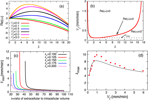
Figure 2. (a) The real part of the eigenvalue  as a function of the wave number k for different flow velocities Vf. (b) A typical shape of the neutral curve (equation (11)) on which
  = 0. Parameters are
  . (c) Critical velocity
  plotted against h for different ke values. (d) k value with maximum growth rate is plotted for different flow rates Vf. The solid line is the result from linear stability analysis and the red dots are obtained from numerical simulations.
  and all the other parameters are given in section 2.
Download figure:
Standard image High-resolution imageAs shown by the bifurcation diagram in figure 3, the parameters σ, ke and h are among the important factors governing the dynamics of the MG model (equations (3)). The region of possible convective instability is labeled CU in the figure where the system can sustain convective instabilities for flow velocities above the critical  . The results in figure 3(a) predict that convective instabilities can occur for both large and small values of h which correspond to lower and higher cell densities, respectively. However, the 'window' for convective instabilities is slightly narrower for larger values of h (low cell density). More importantly, figure 3(b) predicts that, for fixed values of the other parameters, there is a finite range of degradation rate ke just before the absolute unstable (AU) regime, where convective instabilities can occur. This window increases slightly as σ increases (i.e. higher activity of the enzyme adenylate cyclase).

Figure 3. Phase diagram in the (a)  and (b)
  parametric plane showing the region of convective instability (CU) and absolute instability (AU). In the bistable regime (B) of the phase diagram, the system has two stable fixed point of which one is convectively unstable and one is excitable. Stars in figure (b) denote the parameter values for which the simulations in figures 5, 6 were performed. Displayed are the number of stable steady states and the total number of steady states (in parentheses). For the parameters of the model, see section 2.
Download figure:
Standard image High-resolution imageWe solve equations (3) numerically using the Merson modification of the Runge–Kutta method with automatic regulation of the time step. The spatial domain consists of 6000 grid points in the x direction with a mesh size of  mm. The flow is from the left to the right and a no-flux boundary condition is used on the right boundary that corresponds to the outlet of the channel. To have a realistic description of the experiment at the left side of the channel [11], we assume that over the first 2.5 mm of the channel length (corresponding to the inlet of the microfluidic channel), there are no cells and the active production of cAMP drops to zero. cAMP diffuses back from the channel to the inlet area which can then be advected downstream. This boundary condition at the inlet has a significant effect on the observed pattern as will be discussed later.
To show the development of a convective instability along the channel, we select ke = 3 min−1 and  min−1 to be in the CU regime of the phase diagram, but close to transition to AU regime (point
  in figure 3(b)). The flow-driven waves are sustained at flow velocities greater than the critical velocity vmin. In the inlet region, we assume that initially the concentration of cAMP is zero. At t = 0, the spatially uniform steady state of the system is perturbed by slightly increasing the value of γ over a small region in the close neighborhood of the inlet (figure 4(a)). No additional perturbations are applied during the course of the integration. The perturbation applied at t = 0 generates the first wave which propagates along the channel (figure 4(b)). The second wave appears in the downstream of the location where the initial perturbation was applied (figure 4(c)). Note that the new pulse emerge from the back of the already existing pulse, as shown in figures 4(c) and (f). The effect of the refractory tail of the 'mother' pulse is to reduce the amplitude of the 'daughter' wave. As the two wave fronts become more separated, the 'daughter' wave grows to form a fully developed new 'mother' wave. An important feature to note is that each successive wave is formed further downstream than the previous one and the old waves die out as they propagate through the channel (see figure 4). The growth of new wave fronts and decay of the old ones is clearly visible in the corresponding space-time plot presented in figure 5(b). The traveling waves are advected downstream and eventually out of the system with time. The waves initially propagate with velocity of 2.20 mm min−1, which is larger than the imposed flow velocity and as the wave amplitude decays, they slow down to 1.75 mm min−1. Interestingly, the period of the flow-induced waves decrease from 5 to 2.4 min. Similar behavior is observed in figure 5(a) where the parameters are selected to be deep inside the CU regime (point
  in figure 3(b)). Here convective instability waves have smaller amplitudes and the wave package extends over a smaller region of the channel. The bottom two plots in figures 5(c),(d) correspond to simulations in the AU and excitable regime, respectively. The flow driven waves in figure 5(c) are also traveling downstream and interact with uniform bulk oscillations at the lower part of the channel and sweep them away. Note that the boundary condition at the upstream of the channel (zero cAMP concentration) suppresses the bulk oscillations at the upper part of the channel. Similarly, the wave velocity varies from 2.5 to 1.95 mm min−1 before interaction with bulk oscillations and the wave period varies from 5 to 2.5 min. In the excitable regime, if the perturbation amplitude at t = 0 is larger than a critical value, then it is amplified and one single excitation wave propagates along the channel (figure 5(d)), otherwise the perturbation dies out.

Figure 4. Plots of dimensionless concentration γ at t = 0, 4.25, 5.25, 18, 18.5, 19, 19.5, 20 and 20.5 min illustrating the development of a convective instability for the parameter values  and
and  (point ∗2 in figure 3(b)). The perturbation applied at t = 0 develops into wave trains traveling with the flow. Waves caused by the convective instability develop further downstream than those created by the absolute instability. The flow velocity is Vf = 1.5 mm min−1 which is selected to be larger than the critical velocity vmin = 0.44 mm min−1.
Download figure:
Standard image High-resolution image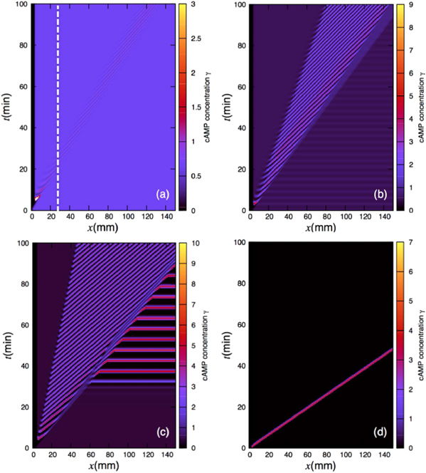
Figure 5. Space–time plots of the dimensionless concentration of cAMP in the (a) convectively unstable regime, (b) convectively unstable regime but close to transition to absolute unstable regime, (c) absolute unstable regime and (d) excitable regime, corresponding to parameter values denoted by 1, 2, 3 and 4 in figure 3(b), respectively. The flow velocity is Vf = 1.5 mm min−1. The dashed line in (a) marks 30 mm channel length in the experiments of [11].
Download figure:
Standard image High-resolution imageFigure 6 shows the results obtained at lower flow velocities, namely Vf = 1 mm min−1. In figure 6(a), the flow velocity is below the critical velocity  mm min−1 and therefore convective instability waves are not observed. However, the cell-free boundary region at the inlet drives a new kind of instability in the area close to the boundary. cAMP secreted by the cells diffuse back to the inlet and at the same time can be advected downstream by the flow. Since there are no cells in the inlet to produce cAMP, the points in the vicinity of the inlet lose cAMP due to advection or diffusion and gain only a little from the upstream of the channel (inlet). In other words, there is a large negative flux of cAMP in the neighborhood close to the inlet, which can be considered as a sink. Under some flow conditions, this sink drives the system from a stable to an oscillatory regime. To obtain a better understanding of sink driven oscillations (SDOs), we performed linear stability analysis of equation (3) for an isolated point with a constant negative flux of cAMP due to advection and diffusion. We also plot the nullclines of equation (3) with zero flux (i.e. no diffusion and no advection) and with negative constant flux of cAMP. Negative constant flux of cAMP shifts one of the nullclines upwards (equation (3a)), but does not change the second nullcline (equation (3b)). Linear stability analysis predicts that for negative flux smaller than a critical value fc, the new fixed point is stable (figures 7(a)–(c)). However, it becomes unstable for a negative flux larger than fc and the system is attracted to a limit cycle (see figure 7(d)). This negative flux can be considered as a driving force for SDOs.
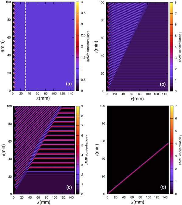
Figure 6. Space–time plots at the same set of parameters as in figure 5 but for a different flow velocity (Vf = 1 mm min−1). (a) The flow velocity is below the critical velocity  mm min−1 and therefore only SDOs are observed in a narrow region close to the inlet. (b) The flow velocity is larger than
  mm min−1 and a combination of flow-driven waves and SDOs are initiated close to the inlet and propagate downstream. (c) Similarly, in the absolute unstable regime, flow-driven waves and SDOs are combined and meet the bulk oscillations at the lower end of the channel. (d) One excitation wave front is initiated from the perturbation site located close to the inlet and is advected downstream. Similar to figure 5, the dashed line in (a) marks the experimental size of the channel [11].
Download figure:
Standard image High-resolution image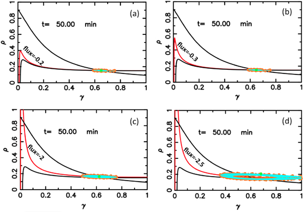
Figure 7. Numerical results of the linear stability analysis and simulations for an isolated point with a constant negative flux of cAMP due to diffusion and advection. This negative flux of cAMP shifts one of the nullclines upwards (red curves) and introduces new fixed point(s). (a)–(c) For the negative flux smaller than critical value −2.4, small oscillations in cAMP concentration damps out and the system is attracted by the new stable fixed point, which is slightly different from the old fixed point. (d) For a negative flux larger than the critical flux, namely −2.5, the new fixed point becomes unstable and a stable limit cycle is the new attractor of the system. The green points in the figures show the current state of the system at t = 50 min and the orange points are the previous states. Parameters are the same as figure 6(a).
Download figure:
Standard image High-resolution imageNext, we run simulations for an extended system (equation (3)) with advection and diffusion for different flow velocities (figure 8). The results are shown for a point located very close to the inlet. At small flow velocities below 0.275 mm min−1, the new fixed point is stable and oscillations in cAMP concentration are damped. It is important to emphasize that e.g. in figure 8(a), at the end the system has a steady negative flux of value −15.3. This negative flux is supposed to destabilize the system, in accordance with linear stability analysis of an isolated point. Interestingly, advection and diffusion stabilize possible oscillations and the system is attracted by the new fixed point. As we increase the flow velocity, at V = 0.275 mm min−1, the shifted nullcline is tangent to the zero-flux nullcline and the system is at the onset of instability (figure 8(b)). Above this critical velocity there is no intersection point anymore, except at very small values of cAMP concentration and a stable limit cycle appears which leads to oscillations in cAMP concentration (see figure 8(c)). In other words, close to the inlet, there is a competition between the destabilizing effect of the inlet and stabilizing effect of diffusion and advection. However, there is an upper limit of flow velocity above which the limit cycle disappears and the system is attracted by the fixed point with small concentration of cAMP (figure 8(d)). For the set of parameters in figure 6(a), SDOs are observed for flow velocities larger than 0.2 mm min−1 but smaller than 1.3 mm min−1. The amplitude of these SDOs decay as the distance to the inlet region increases. Far away from the inlet, the net flux of cAMP is very close to zero and the new fixed point is stable.
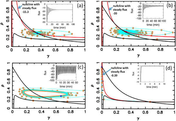
Figure 8. Numerical simulations of equations (3) with advection and diffusion for a point located close to the inlet. (a) For V = 0.25 mm min−1, the system reaches a negative steady flux of −15.3 which based on the linear stability analysis is predicted to destabilize an isolated system. However diffusion and advection stabilize this point and oscillations damp away. (b) At the flow velocity of V = 0.275 mm min−1, the system is at the onset of instability. The flux shows tiny oscillations around -20 and the new shifted nullcline with steady flux of −20 is tangent to the zero-flux nullcline. (c) By increasing the flow velocity to 0.3 mm min−1, the new nullcline has only one intersection point with the zero-flux nullcline and a stable limit cycle is appeared. (d) At high flow velocity of 1.3 mm min−1, cAMP is washed away and the only attractor of the system is the fixed point with small concentration of cAMP. The blue points in all the figures present the state of the system at t = 100 min and orange points are the previous states. Parameters are the same as figure 6(a).
Download figure:
Standard image High-resolution imageIn figure 6(b), the SDOs are combined with flow driven waves, where the flow velocity is well above the critical velocity  mm min−1. Similarly, a combination of SDOs and flow-driven waves is observed in figure 6(c), which is very similar to the experimental observations in [11]. In the experiments, the channel length was only 30 mm. Thus figure 6(c) predicts that for experiments with much longer channels, uniform bulk oscillations may be observed at the downstream of the channel.
4. Linear stability analysis and numerical simulations of the three-component MG model
In this section, we consider the full set of equations with diffusion and advection (equations (1a), (1b) and (2)). If we assume that the system has a stable steady state  , then the evolution of a small perturbation is governed by the linearized equations


where

where  are small and aij are the elements of the Jacobian matrix


with M0, N0, A0 and B0 defined in equation (7).
We first consider the system without diffusion and convection and introduce the following definitions:  is the trace of the system, Δ is its determinant,
  is the trace of the subsystem formed by
  or
or  or
or  , and
, and  is the determinant of the same subsystem, while
  . Based on the Hurwitz criterion [25], the stability of the entire three variable system requires that

Let us now consider the system (12) with flow but without the diffusion term. We represent the perturbations  by the spatial Fourier transform
  . The equations for the Fourier components then become


We form the characteristic polynomial  , where ω, PR, and PI are all real. The real and imaginary parts of
  are
are


For convective instability to occur, the following conditions should be fulfilled [2]

where  .
.
Including the diffusion of extracellular cAMP in addition to the convection term generates a short wavelength cutoff in the dispersion relation and leads to the appearance of a critical velocity, similar to the two-component case. We used the criteria in equation (18) to explore the regions of convective instabilities in the  and
and  parametric planes (see figure 9). Note that again, similar to the two-component MG model, regions of CU occur right before the absolute instability (AU) but in a narrower region (figure 9(b)).
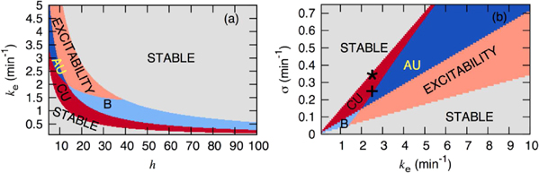
Figure 9. Phase diagram of the three-variable MG model in the (a)  and (b)
  parametric plane showing the region of convective instability (CU) and absolute instability (AU). Similar to the two-variable MG model, one of the two existing stable fixed points in the bistable regime (B) is convectively unstable and the other one excitable.
Download figure:
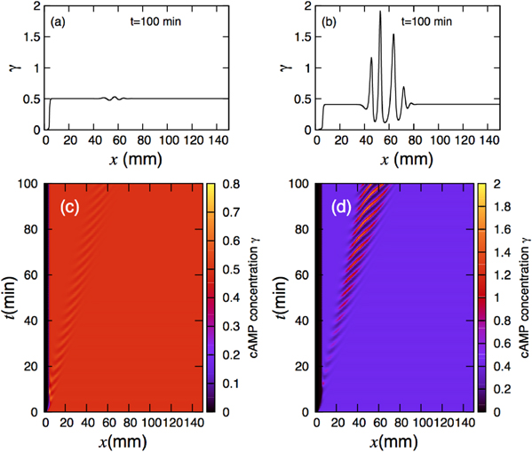
Standard image High-resolution imageWe extended the numerical simulations described in section 3 to the three-component MG model and performed simulations for the set of parameters inside the CU regime, namely  and
and  . This point is marked by the ⋆ symbol in figure 9(b) and is located close to the transition line but in the convectively unstable region of the phase diagram. Note that, in the absence of flow (and diffusion), the homogeneous steady state is stable to small perturbations; however an external flow above the threshold velocity vmin may lead to convective instability. The corresponding wave pattern is illustrated in figures 10(a), (c). Remarkably, the flow driven instability waves of cAMP need more time to be fully developed. Since the system is very close to the transition line to the stable region, the wave fronts have a lower concentration of cAMP. However, deep inside the CU regime and close to the lower transition line in figure 9(b), the instability waves appear earlier in time and have higher concentrations of cAMP (see figures 10(b), (d)). This point is denoted by + in figure 9(b) and corresponds to parameter values
  and
and  .
.
Figure 10. (a), (c) Numerical simulations of the three-component MG model in the vicinity of the transition line to the stable regime, denoted with ⋆ in figure 9(b). Notably, convective instability waves propagate slower and wave fronts have lower concentrations of cAMP than in the two-component MG model. (b), (d) Instability wave patterns for the parameters right before the transition to the absolute unstable (AU) regime denoted by + in figure 9(b). The flow velocity is Vf = 1.5 mm min−1.
Download figure:
Standard image High-resolution image
5. Discussion
Our linear stability analysis and numerical simulations of the MG model have shown that an advective flow of extracellular cAMP through a uniform field of signaling D.d. cells can induce a pattern forming instability. We found that, in the convectively unstable regime, small perturbations in the concentration of cAMP grow in the course of time and generate a wave train moving only in the flow direction. The flow-driven instability presents a non-oscillatory state without fluid flow that develops a pattern if the flow velocity increases beyond a critical threshold. We have repeated our numerical simulations for different flow rates and measured the wave propagation velocity as well as the wavelength. The calculated wave velocity and wavelength for different flow rates follow a linear relationship which is in agreement with experimental observations in [11]. However, the convective nature of this instability which is recognized in the numerical simulations as well as in linear stability analysis, is not directly observed in the experiments. Moreover, there are important experimental features that are different from numerical simulations. In the experiments, the propagating flow-driven waves appear to fill the whole length of microfluidic channel. This is different from simulations where each new wave front is formed further downstream than the previous one. Perhaps this is due to small continuous inlet-perturbations which exist throughout the experiment and can be considerably amplified by convective instabilities. These time-dependent inlet perturbations are not included in the numerical simulations where only a single perturbation was applied as an initial condition. Another possible explanation is the effect of the boundary which leads to a new kind of instability close to the inlet. As discussed in great detail in section 3, SDOs initiate the wave patterns in the vicinity of the inlet which is more similar to our experimental observations in [11]. This suggests that wave patterns observed in the experiment, could be a combination of flow-driven waves and SDOs. In addition, there is a significant difference between the experimental system which is a living system under development and the system studied numerically. In the numerical simulations, the point selected in the convectively unstable regime of the phase diagram is stable when the external flow is switched off and always remains at the same place in the phase diagram. However, D.d. amoebae represent a system, which is under continuous development and in the absence of external flow, they synchronize and show formation and propagation of spiral waves. In other words, in the course of development, the living system can have a developmental path in the phase diagram as has been proposed in [26].
There are relevant biological questions related to the influence of flow-driven waves on aggregation pattern of D.d. cells. These waves are observed in the initial stages of cell signaling, where the cell population is assumed to have a uniform distribution. However as the cells start to aggregate, variations in the cell density become significant. Future studies should attempt to include chemotactic cell movement in the simulations to study the distribution of cell population in the presence of flow-driven waves. Our results may also provide a starting point for the study of pattern formation and locomotion-driven instabilities in other biological systems.
Acknowledgments
We are grateful to Alan Pumir for discussions and comments. A G was supported by Dorothea-Schlözer scholarship from Georg-August University of Göttingen, Germany. O St acknowledges support provided by the A v Humboldt Foundation and the National Science Foundation (CHE-1213259).