


Abstract
Turbulent pair dispersion of heavy particles is strongly altered when particles of two different Stokes numbers (bidisperse) are considered, and this is further compounded when a uniform gravitational acceleration is present. Lagrangian trajectories of fluid tracers, and bidisperse heavy particles with and without gravity were calculated from a direct numerical simulation of homogeneous, isotropic turbulence. Particle pair dispersion shows a short-time, ballistic (Batchelor) regime and a transition to super-ballistic dispersion that is suggestive of the emergence of Richardson scaling. A simple equation of motion for inertial, sedimenting particles captures the essential features of the pair dispersion at very short time and length scales. Kolmogorov scaling arguments are able to qualitatively describe the competition between gravity-induced and fluid-induced relative motion in modifying the amount of time the heavy particles spend in the ballistic regime. The transition from ballistic to super-ballistic dispersion for fluid tracers and monodisperse inertial particles exhibits a pronounced sub-ballistic behavior that can be attributed to the mixed velocity–acceleration structure function. The sub-ballistic behavior is strongly suppressed for bidisperse particles, both in the presence or absence of gravity, primarily because of a reduction in the correlation between velocity and acceleration increments.
Export citation and abstract BibTeX RIS

Content from this work may be used under the terms of the Creative Commons Attribution 3.0 licence. Any further distribution of this work must maintain attribution to the author(s) and the title of the work, journal citation and DOI.
1. Introduction
One defining characteristic of turbulent flow is its efficiency of mixing, which may be expressed as the rapid dispersion of pairs of fluid elements. It has been shown theoretically, computationally, and experimentally that pair dispersion begins with a ballistic separation rate known as the Batchelor regime (see e.g. [1–3]). This short-time behavior is followed by a transition to a super-ballistic separation rate, usually considered the Richardson regime [4], although there is a paucity of computational or experimental evidence for strict Richardson scaling. When fluid elements are replaced with small, identical particles that are heavy compared to the surrounding fluid (inertial particles) the nature of dispersion is slightly altered (e.g. [5, 6]). These inertial particles are known to cluster in high strain regions [7, 8], suppress violent acceleration events [9, 10], and have non-vanishing velocity difference at small separations (a result which is linked to crossing trajectories that are responsible for the enhancement of the collision probability in turbulent flow, see [11–13]). In this paper we consider the role of a constant gravitational acceleration, which can represent any steady, spatially uniform body force, on the pair dispersion of inertial particles; furthermore, we consider particles with different inertia (here referred to as 'bidisperse', as opposed to 'monodisperse'). The presence of gravity results in a steady separation rate aligned with the gravity coordinate for particles falling at terminal velocity, so this already can be seen to alter the rate of, and perhaps even the nature of the pair dispersion.
Our study is motivated by the practical problem of the behavior of droplets in clouds, ultimately with interest not only in their collision rate to form precipitation, but also in their interaction with surrounding scalar fields such as temperature and water vapor concentration. The interplay between droplets and the flow and thermodynamic environment influences the energetics of the atmosphere through phase changes and radiative transfer, and the distribution of precipitation, so the problem is of considerable practical relevance beyond its inherent aesthetic and intellectual merit. The parameter space corresponding to the inertial particle dispersion problem is enormous, so we use atmospheric clouds as a context for restricting the region of study within that space: particles small compared to the Kolmogorov length scale, heavy compared to the surrounding fluid, and obeying to good approximation a linear (Stokes) drag law. Significantly, from the point of view of this study, clouds consist of a population of condensing or evaporating water droplets advected by turbulent air flow in a thermodynamically varying environment, with the result that the size distribution of droplets can be quite broad [14]. There is considerable computational and experimental evidence already that different sizes and therefore different inertial response, can lead to significant changes in the behavior of inertial particles. For example, the tendency to cluster weakens in the case of inertial particles with a broad size distribution (e.g. [15, 16]). Furthermore, the dynamics of this polydisperse population of particles can be significantly modified by the presence of a gravitational acceleration that results in particle decoupling from the fluid motions, and perhaps more importantly, a relative velocity of different-sized particles falling at terminal speed [17, 18]. Simple Kolmogorov dissipative range scaling arguments (e.g. [19]) suggest that the mean turbulent acceleration in clouds is in the approximate range of 0.1–1 m s−2, much less than gravitational acceleration. This has the consequence that gravity very likely has an immediate effect on the dispersion of polydisperse droplets in the atmosphere [20]. The emphasis of this work is to explore the role of gravity in turbulent pair dispersion for conditions relevant to clouds. In particular, we emphasize the influence of gravity and of differential inertia (i.e., bidisperse particles) on the transition from ballistic to super-ballistic dispersion. We organize the paper as follows. Section 2 reviews simplified governing equations for heavy particles. This is followed by section 3 in which we describe the numerical approach to simulate turbulent pair dispersion. We discuss the simulation results and compare them to theoretical predictions in section 4. Finally, we summarize our findings in section 5.
2. Theoretical background
Our analyses rest upon the theoretical framework of Maxey and Riley [21], who derived the most general equation of motion describing particles with size smaller than the smallest eddy length scale of the flow and with small particle Reynolds number. Neglecting the buoyancy force, the Basset history force, and the added mass term, the equations are


Here,  and
and  are the particle position and velocity vectors, respectively,
  is the fluid tracer velocity,
  is gravitational acceleration, and τ is the particle inertial relaxation time. The operator
  indicates a derivative along the particle trajectory. Let us introduce the following dimensionless variables:
  for time,
  for space, and
  for velocity, where
  is the Kolmogorov time scale,
  is the Kolmogorov length scale,
  is the Kolmogorov velocity scale, ν is the kinematic viscosity and
  is the energy dissipation rate. We define the following dimensionless numbers:
  for the Stokes number, and
  for the dimensionless gravity, where
  is the Kolmogorov acceleration scale, so that upon rearranging equation (2) we obtain

where  is the vertical unit vector. We shall work in the limits of small particle inertia (
 ) and strong external field (
 ), so that the particle acceleration,
  , in equation (3) can be treated as a small perturbation to the zeroth order solution
  . Inserting this initial solution into equation (3) yields

where  is the dimensionless fluid acceleration. Let us estimate the relative order of the last two terms by considering the vertical component of the equation. The vertical acceleration has a variance of
  , where a0 is the Heisenberg–Yaglom constant [22, 23] whose typical value is about 4, whereas for the vertical gradient, its variance is
  , according to Taylor [24]. The ratio of the acceleration term to the gradient term is thus
  . Based on this estimate, we may neglect the gradient term and consider only the following approximation for the particle velocity, in dimensional form

Equation (5) is the simplest solution to the particle equation and is frequently employed to describe the effect of particle inertia in the limit of small Stokes number (e.g. [20, 25]).
2.1. The pair dispersion
Let us define the particle pair separation  , the separation increment
  , and the relative velocity
  . Following the work of Batchelor [1], the Taylor expansion of the particle pair dispersion
  in the short-time limit is

where  is the heavy particle Eulerian second order structure function and r0 is the initial separation. The brackets
  indicate an ensemble average over all particle pairs along their trajectories. The monodisperse case has been considered by Bec et al [5], Gibert et al [6] and Salazar and Collins [26]. Here, we treat the bidisperse case and include gravity in our analysis. In the following section, we show that for small separations the effect of gravity on bidisperse particle pair dispersion is an additive term in the particle structure function.
2.2. The structure function
Obtaining the structure function requires formulating the relative velocity  using equation (5) for bidisperse particles, which we obtain as follows

where  . The appearance of
  necessitates the set of transformations
  ,
,  , and
, and  , so that
  can be expressed as
  . Upon squaring
  and averaging it over an ensemble of particle pairs, we arrive at
We shall analyse S(r) in the dissipation range,  , because these length scales are most relevant to the cloud droplet collision problem. In this regime, we can apply the dissipation-range scaling for the fluid tracer structure function (see e.g. [19]),
  .
.
Equation (8) contains the variance of the mean acceleration term,  , which for fluid tracers reduces to
  , where a0 is the Heisenberg–Yaglom constant [22, 23]. The case for bidisperse inertial particles does not permit simple analysis. We could, however, obtain some qualitative understanding from the monodisperse case. As noted by various authors experimentally and numerically, see e.g. [9, 10, 27], inertial particle acceleration variance decreases monotonically with Stokes number from fluid tracer acceleration variance. This behavior is attributed to two effects: preferential sampling of inertial particles in regions with high strains and low vorticity, and filtering of high-frequency fluctuations effected by the selective response of the inertial particles to temporal rate of change in the acceleration. In our problem, because the operation
  involves taking the average along inertial particle trajectories, preferential sampling must necessarily play a role in determining the value of
  .
.
The term  , which is known to asymptote to the value
  in the inertial range (see e.g. [28–30]), has no known analytical expression in the dissipation range. By use of reasonings in the same vein as Kolmogorov's, we anticipate, however,
  to scale as r2 in the dissipative range of scales. We note that the variance of the acceleration increment is connected to the acceleration correlation by the relation
  . Obukhov and Yaglom [31] have shown that
  approaches simple scaling laws r2 in the dissipation range. In this connection,
  may contain similar scaling laws. The remaining terms containing
  ,
,  ,
,  ,
,  and
and  vanish for fluid tracers in isotropic and zero mean flow. Whether these approximations are reasonable is addressed in section 4.2.
3. Numerical methods
Our simulations can be classified into three distinct types. They are (a) fluid tracers, (b) bidisperse heavy particles in the absence of gravity, and (c) bidisperse heavy particles in the presence of gravity. For all cases, the particle motion is driven by fluid motions obtained from the Johns Hopkins University (JHU) simulation of a forced homogeneous isotropic turbulence in stationary state at a Taylor Reynolds number,  , of 433 on a
  numerical domain [32]. The basic flow properties are summarized in table 1. For fluid tracers we solve only equation (1), with
  taken from the JHU direct numerical simulation (DNS). For non-fluid tracers, we solve both equations (1) and (2) numerically for a population of bidisperse particles. In all cases, the particles are initially arranged on
  grids with a uniform spacing of 0.004, approximately
  . We consider four pairs of Stokes numbers; they are 0.1 with 0.5, 0.2 with 0.4, 0.4 with 0.5, and 0.8 with 0.9. The Stokes number alternates between the smaller value and the larger one for adjacent pairs. Within the particle grid, there are 63 particles with the small Stokes number and 62 particles with the large Stokes number.
Table 1. Some basic flow properties of the Johns Hopkins turbulence database. All values are in simulation units.
| Flow variable | Symbol | Value |
|---|---|---|
| Reynolds number |

|
433 |
| Energy dissipation rate |
|
0.0928 |
| Viscosity | ν | 0.000 185 |
| rms velocity | u' | 0.681 |
| Total simulation time | TS | 2.048 |
| Integral time | TL | 2.02 |
| Integral length | L | 1.376 |
| Taylor length scale | λ | 0.118 |
| Kolmogorov time scale |

|
0.0446 |
| Kolmogorov length scale | η | 0.002 87 |
In simulating particles in the presence of gravity, the strength of gravity is ten times the Kolmogorov acceleration,  . This magnitude is chosen for its relevance to the cloud droplet problem [14] and to satisfy the condition
  (see section 2). Fluid tracers and heavy particles in the absence of gravity are initialized with fluid tracer velocities
  . Heavy particles in the presence of gravity have terminal velocities added to their initial fluid tracer velocities, so that the initial velocities are
  . The time steps for the propagation of positions and velocities are
  for fluid tracers,
  for
for  , and
, and  for
for  . We solve the first two time steps of the particle equations using the fourth-order Runge–Kutta method [33]. Thereafter, the particle trajectories for the remaining time steps are calculated using an Adams–Bashforth third-order method [33]. Because the temporal and spatial grid points of the JHU DNS are uniformly spaced and the resolutions are 0.0002 and
  in time and space, respectively, in order to obtain particle positions at time steps lying outside of the numerical grid, numerical interpolation is needed to achieve subgrid resolution. We used a piecewise cubic Hermite interpolation for the temporal interpolation and a sixth-order Lagrangian interpolation for the spatial interpolation. These interpolations are implemented on the JHU computational server.
Because the flow is isotropic, we only sample the flow at 125 locations around the neighborhood of the diagonal in one octant of the numerical domain. Overall, we follow the trajectories of 15 625 particles starting from the initial simulation time at t = 0 and up to t = 2, which is approximately one large eddy turn over time. To estimate the accuracy of the trajectories, we calculate a trajectory multiple times with the same initial conditions and time step, and look for any difference between trajectories from different runs. We find that the difference is no more than 10−6 (in simulation units) for the positions, and 10−5 for the velocities, whose origin can be traced to the numerical noise arising from the various spatial and temporal interpolation schemes. The velocities and accelerations have negligible mean (not shown) that only affect the statistics reported in this work by no more than 1%. Also not shown are the second-order Lagrangian velocity structure function and the acceleration probability distribution of the flow, which we have compared and are fully in agreement with the results published by the JHU database [34] and elsewhere.
4. Results and discussion
We organize our main results as follows. In sections (4.1) and (4.2) we present pair dispersion and structure function results, respectively, and compare them to theoretical expressions. In section 4.3 we consider the transition from ballistic to super-ballistic dispersion for particles with gravity. And in section 4.4 we consider the role of the mixed velocity–acceleration structure function in the transition.
4.1. The pair dispersion
We show in figure 1 the pair dispersion,  , of bidisperse heavy particles (St = 0.1 and 0.5) in the presence and absence of gravity, as well as that of fluid tracers. The statistics are collected the instant the particles are initialized. In all three cases,
  scales quadratically with t at short time, in agreement with the Batchelor prediction, as expressed in equation (6). The simulation also confirms that, in the dissipation range, heavy particles in a turbulent flow experiencing gravity separate faster than both fluid tracers and heavy particles without gravity. The essential features of the short-time behavior is captured by the particle structure function, which we discuss in the following section.
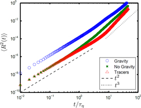
Figure 1. The pair dispersion,  , for passive tracers
  , bidisperse heavy particles (St = 0.1 and 0.5) in the absence of gravity (×), and bidisperse heavy particles in the presence of gravity (◯). The dashed line is proportional to a t2 power law, whereas the dotted line is proportional to t3.
Download figure:
Standard image High-resolution image4.2. The structure function
In calculating the structure function, fluid tracer statistics are collected immediately after initialization, while heavy particle statistics are collected only after they have relaxed to a stationary state (typically two relaxation time of the heavier particle after initialization). We have numerically investigated the individual correlations appearing in equation (8) for fluid tracers, the details of which could be found in the supplementary material document. We briefly summarize the results of the our investigation as follows. We find that the most significant term is the acceleration variance,  , which we estimated, following the approach of Bec et al [9], by calculating the fluid tracer accelerations measured along inertial particle trajectories for separations in the range
  . The values of
  for various pairing of the Stokes numbers calculated with this approach are shown in table 2. All the variances are below the isotropic limit
  , whose value in our flow is approximately 11.6. These values of
  are in qualitative agreement with those estimated by taking the average between the variances for the monodisperse case calculated with the expressions derived by Ayyalasomayajula et al [27] and Zaichik and Alipchenkov [35]. Two additional terms contribute to S(r), namely
  and
and  , whose scaling in the dissipation range we have empirically determined to follow the power laws
  and
and  , respectively (see supplementary material document for further details). The remaining terms
  ,
,  ,
,  ,
,  and
and  are found to have negligible contributions. Using these empirical results, we can derive the following expression for the structure function

valid only for separations in the range  . In the above expression, the linear
  term originates from the correlation
  , whereas the
  term can be traced back to the term
  . It is worthwhile to mention that both contributions from
  and
and  are essentially negligible for
  .
.
Table 2.
The acceleration variance  , in units of
  , measured along the trajectories of bidisperse inertial particle pairs.
| Stokes number pairing | 0.1 and 0.5 | 0.2 and 0.4 | 0.4 and 0.5 | 0.8 and 0.9 |
 |
4.3 | 3.1 | 3.3 | 2.9 |
We test equation (9) for fluid tracers, and for heavy particles in the absence and presence of gravity in figure 2. Although not visible on a logarithmic plot, the fluid tracer structure function is exactly zero at zero separation. The measured structure functions for heavy particles, however, maintain a positive offset at zero separation. In the insets, we show the data for the structure function in more detail by dividing out the prediction from equation (9). It is interesting to note that beyond the slight change in  the structure function is insensitive to
  , as evidenced by the Stokes number pairs 0.4 with 0.5, and 0.8 with 0.9. The
  in both cases are the same, but their
  are significantly different, 0.45 and 0.85, respectively. Remarkably, not only the numerical results are indistinguishable from each other, but they agree with the highly simplified expression, equation (9). At increasing separation distances,
  , the simulation data start to deviate from the prediction. We believe the deviation is due to the dissipation and inertial range transition dynamics, which is not captured by our dissipation range model.

Figure 2. The normalized structure function  for bidisperse particles (a) in the absence of gravity and (b) in the presence of gravity, for various Stokes number (St) pairs. Symbols are simulation results, solid and dotted lines are the predictions from equation (9). In panel (b), the magnitude of gravity is
  . The St = 0 case refers to fluid tracers. The insets show the same structure functions divided by their predictions from equation (9), as a function of
  .
.
Download figure:
Standard image High-resolution imageWe digress a bit by noting that the expression in (9) bears some resemblance to the gravitational settling collision rate of Saffman and Turner [36], and to the diffusivity tensor considered by Chun et al [37]. We can establish the link between the velocity structure function and the collision rate,  , starting with the canonical form for the collision rate

where n1 and n2 are the mean number concentrations of droplets with two distinct radii r1 and r2 respectively,  is the relative velocity of the pair just before they collide (which is
  in our notation), and
  is the probability distribution of the relative velocities. The integral involving the relative velocity is evaluated over the entire space. Under the assumption that
  is normally distributed, Saffman and Turner showed that this integral can be integrated to yield a collision rate

where S is the structure function given by equation (9), without the  corrections, evaluated at
  .
.
The relationship between the structure function and the diffusivity, defined as

is less apparent, but can be understood if we consider its short-time behavior. For time scale much shorter than the correlation time of the relative velocities,  , the two-time two-point correlation
  is approximately equal to the single-time structure function,
  , and the diffusivity is approximately
  (see e.g. Falkovich et al [38]). This implies that the spatial information of the diffusivity is fully contained within the structure function, whereas its temporal information is described by the relative velocity correlation time. Along the same line of analysis, Lu et al [39] extended the theory of Chun et al [37] to include the contribution of gravity and the diffusivity tensor they derived is, up to a multiplicative constant, identical to the expression shown in equation (9).
The foregoing analysis reveals three points about turbulent pair dispersion of bidisperse heavy particles, as summarized in equations (6) and (9). First, the separation of bidisperse particles in the presence of gravity at short time scales remains ballistic. In other words, the square of the separation increment is quadratic in time. Second, the particle differential response to gravity and fluid acceleration at short time scales is fully described by the particle structure function. Third, gravity contributes to the dispersion of heavy particles with the same order of the differential Stokes number as the fluid acceleration. It is perhaps illuminating to mention that in the parameter space we considered, gravity dominates over the fluid acceleration, so that the largest contribution to the dispersion of heavy particles is from gravity.
We note that this result for the structure function is not applicable to the monodisperse case, which has been treated by Gibert et al [6] and Salazar and Collins [26]. Gibert et al [6] measured the pair dispersion of monodisperse solid spherical particles in a laboratory experiment with fully developed turbulence in water at a Taylor Reynolds number of 442. They observed a Batchelor regime in the early stages of the relative motion of particle pairs. Their measurement shows that particle inertia increases the particle structure function but leaves the short-time ballistic scaling unchanged. Salazar and Collins [26] studied pair dispersion in a DNS of homogeneous isotropic turbulent flow laden with monodisperse heavy particles in the absence of gravity and at a Taylor Reynolds number as high as 120. For Stokes numbers 0.2 and higher, their simulations showed that the particle structure function consistently retains a constant positive offset from that of the fluid for separations in the dissipation range. The simple model presented here is unable to predict this offset. Whether it is therefore able to capture the early dispersion is open to question, and is addressed in the next section.
4.3. The transition time
In a paper that preceded the work of Batchelor [1], Obukhov [40] applied Kolmogorov's dimensional argument to explain Richardson's empirical scaling [4] for turbulent pair dispersion,  , valid only in the inertial range of scales. Fluid particles in turbulence are understood to separate ballistically at very short time and gradually transition to the Richardson regime at later time. This change in the separation rates influences, for example, the droplet collision rates and the chemical mixing rates. It is intriguing to investigate whether the presence or absence of gravity affects this transition. We present our measurement of the heavy particle pair dispersion, normalized by the Batchelor short-time solution given by equation (6), in figure 3.

Figure 3. The pair dispersion, normalized by the Batchelor ballistic term, for bidisperse and monodisperse inertial particles (a) in the presence of gravity and (b) in the absence of gravity.
Download figure:
Standard image High-resolution image
The figure shows that particles both with and without gravity separate ballistically for very short time but the Batchelor regime for heavy particles in the presence of gravity persists for a longer time than that for heavy particles in the absence of gravity or for tracers. At time scales of the order of the Kolmogorov time, the particles transition into a non-ballistic regime, whose scaling with time we are unable to ascertain accurately due to the limitation in the simulation time.
Qualitatively, we can understand the extension of the ballistic regime for particles experiencing differential sedimentation through the following heuristic argument. The Batchelor regime is defined by selecting the eddy turnover time corresponding to the initial particle separation distance r0 (assuming the initial separation lies within the inertial range), such that  . Alternatively, by Kolmogorov reasoning, we could replace the initial separation with
  , where
  is the initial differential velocity, to yield
  . We can define a differential settling velocity,
  , to obtain a 'gravitational Batchelor time'

In effect, particles of different size and therefore different terminal speed, are expected to separate ballistically by differential sedimentation until they reach a separation distance at which the corresponding eddy velocity is equal to that sedimentation velocity. At larger scales the turbulent velocity becomes dominant in the pair dispersion. For the bidisperse particles in our simulation  , whereas
  . A curve fit to the observed dispersion curves indeed shows that the transition from the linear to higher-order terms occurs at approximately
  for the bidisperse particles in the presence of gravity, whereas for both tracers and bidisperse inertial particles without gravity the transition time is approximately
  . This lends at least semi-quantitative support to the notion of a gravitational Batchelor time for the transition from ballistic to super-ballistic dispersion.
4.4. Mixed structure function
An intriguing feature of figure 3 is the rather distinct change in the negative dip to sub-ballistic dispersion: the pronounced negative dip observed for the tracers nearly disappears for bidisperse inertial particles both with and without gravity. The initial transition to sub-ballistic dispersion for tracers has been observed in experiments by Ouellette et al [2], and they attributed it to the t3 term in the Taylor expansion of the tracer pair dispersion

Equation (14) contains the mixed structure function  . Mann et al [28, 29] and Hill [30] have shown that
  within the inertial range, thereby explaining the negative behavior. The simulation results presented here show not only the temporary sub-ballistic excursion, but the eventual transition to super-ballistic behavior, presumably due to still higher-order terms in the Taylor expansion. How does the presence of particle inertia and gravity change this behavior?
We gain further insight into this transition by considering both mono and bidisperse particle pairs, in comparison with fluid tracer pairs. It is immediately evident from inspecting figure 3 that monodisperse particles with inertia or with gravity still show pronounced sub-ballistic regimes prior to entering the super-ballistic regime. In contrast, both with and without gravity, the bidisperse particles exhibit strongly suppressed sub-ballistic behavior. Especially for the no-gravity case, there is little difference in the dispersion curves for fluid tracers and for inertial particles; similar can be said for fluid tracers and St = 0.1 monodisperse particles. Dispersion of bidisperse particles shows a more rapid onset of super-ballistic behavior with and without gravity, as compared to fluid tracer and all monodisperse particles; as was observed in the figure 3, bidisperse particles without gravity are fastest to transition to super-ballistic dispersion.
To quantify the very different behavior for bidisperse particles we have computed the zero-time mixed structure function, and to allow for meaningful comparison we have scaled it by the second-order velocity structure function. Particle accelerations in the mixed structure function are obtained with the gaussian filtering and differentiation technique (e.g. [41]). It should be noted that the initial pair separation is not the same for all cases: it is  for tracer and bidisperse particles, and is
  for monodisperse particles. The results for all particle-pair cases are displayed in the dimensionless form
  in table 3. The largest magnitude is for fluid tracers, and both with and without gravity there is a decrease in magnitude with increasing
  . The values for monodisperse particle pairs of a given
  are nearly the same with and without gravity, and for St = 0.5 the scaled mixed structure function is approximately a factor of 10 smaller than for tracers. In other words, with quite negligible influence of gravity, the mixed velocity–acceleration structure function decreases in magnitude relative to the second-order velocity structure function with increasing particle inertia. Bidisperse particles without gravity have a value that is essentially the mean of the two monodisperse values. This is somewhat surprising given the observation from figure 3(b) that bidisperse inertial particles without gravity exhibit very different transitions from the ballistic to super-ballistic dispersion regimes. Finally, in contrast to the no-gravity case, bidisperse particle pairs in the presence of gravity have the smallest magnitude observed for the scaled mixed structure function.
Table 3.
The normalized coefficients for the linear-t term in the expansion of  for fluid tracers, bidisperse (St = 0.1 and 0.5), and monodisperse inertial particles.
| Gravity | Stokes number |

|

|
|---|---|---|---|
| 0 | 0 | 0.132 | −0.1131 |
| 0 | 0.1 and 0.5 | 0.0204 | −0.0283 |
| 0 | 0.1 | 0.0404 | −0.147 |
| 0 | 0.5 | 0.009 54 | −0.153 |
 |
0.1 and 0.5 | 0.005 14 | −0.0325 |
 |
0.1 | 0.0418 | −0.150 |
 |
0.5 | 0.0122 | −0.136 |
The observed behavior of the mixed structure function for the different cases could be the result of changes in the scaling factor  , the magnitude of the acceleration increment
  , or changes in the correlation between velocity and acceleration increments
  . The latter is perhaps most insightful, and we show the zero-time correlation coefficient
  in table 3. Perhaps surprisingly, it is observed that monodisperse inertial particles exhibit stronger anticorrelation than do tracers. This is opposite to the observed trend for the scaled mixed structure function. Both with and without gravity, the correlation coefficient for velocity–acceleration increments diminishes significantly in magnitude (i.e., the anticorrelation becomes weaker) compared to tracers and to monodisperse inertial particles also with and without gravity. The strong decorrelation that results for bidisperse particles is very likely the cause of the striking difference in transition behavior observed in figure 3. We can speculate that the decorrelation is related to that observed in inertial particle clustering, for which it has been clearly observed in simulation and experiment that increasing the gap between the inertial response of particles of two different St induces the two populations to move independently from each other, thereby reducing the overlap between individual clusters (as measured through the radial distribution function) [15, 16]. Even when inertial particles of two different St exhibit considerable self-clustering, the spatial locations of the clusters are not collocated, and therefore the bidisperse correlations are diminished. In the dispersion problem this apparently results in a suppression of the sub-ballistic behavior and an earlier transition to the super-ballistic regime.
5. Discussion and summary
Several open questions remain. The long-time pair dispersion is clearly super-ballistic and is suggestive of the emergence of Richardson scaling, but higher Reynolds numbers are necessary in order to draw a definitive conclusion. Our simple model, while capturing important aspects of the dispersion, is deficient for the monodisperse case. Perhaps the greatest challenge is in returning to the initial motivation for the work, to understand the role of gravity and particle bidispersity in determining the relative motion of heavy particles in turbulence, as for example is relevant to the collision rate of particles in atmospheric clouds. It is clear that bidispersity profoundly alters not only the short-time behavior, but also the transition to long-time, super-ballistic dispersion.
The work presented here highlights the role of gravity and fluid acceleration in the turbulent pair dispersion of particles. Emphasis is placed on bidisperse particles, for which inertia and gravitational acceleration lead to additional sources of relative velocity, and therefore contribute to the transition from ballistic to super-ballistic dispersion regimes. A relatively simple particle equation of motion has been shown to provide insight into the turbulent pair dispersion of heavy particles with bidisperse size distributions. Both model and numerical simulation show that, because of the particle differential response to local acceleration, at length scales relevant to the droplet collision problem, it is reasonable to assume that gravity and fluid acceleration contribute additively to the particle structure function, while leaving the short-time scaling behavior of the pair dispersion unchanged. In addition, both gravity and fluid acceleration compete in a non-trivial way to modify the amount of time the particles spent in the short-time Batchelor regime. A simplified argument based on the Kolmogorov scaling argument qualitatively describes the difference between the gravity and non-gravity case but is unable to yield a more quantitative agreement with the numerical results. Finally, the simulations clearly show a significant change in the behavior during transition from ballistic to super-ballistic dispersion: specifically, the 'negative dip' observed for fluid tracers and monodisperse particles essentially disappears for bidisperse particles, both in the presence and absence of gravity. This is likely a result of a reduction in the correlation between velocity and acceleration increments for bidisperse particles.
Acknowledgments
This work was supported by the US National Science Foundation grant AGS-1026123. The fluid tracer data is obtained from the Johns Hopkins University turbulence database cluster at http://turbulence.pha.jhu.edu. We thank F Nordsiek for assistance with the initial setup of the computations and for many insightful discussions throughout this work, and we acknowledge helpful discussions with E Bodenschatz, N Ouellette, EW Saw, and J Bec in the interpretation of the results.