Abstract
Fast and accurate quantum operations of a single spin in room-temperature solids are required in many modern scientific areas, for instance in quantum information, quantum metrology, and magnetometry. However, the accuracy is limited if the Rabi frequency of the control is comparable with the transition frequency of the qubit due to the breakdown of the rotating wave approximation (RWA). We report here an experimental implementation of a control method based on quantum optimal control theory which does not suffer from such restriction. We demonstrate the most commonly used single qubit rotations, i.e.  - and π-pulses, beyond the RWA regime with high fidelity
 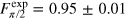 and
and 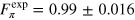 , respectively. They are in excellent agreement with the theoretical predictions,
 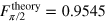 and
and 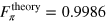 . Furthermore, we perform two basic magnetic resonance experiments both in the rotating and the laboratory frames, where we are able to deliberately 'switch' between the frames, to confirm the robustness of our control method. Our method is general, hence it may immediately find its wide applications in magnetic resonance, quantum computing, quantum optics, and broadband magnetometry.
Export citation and abstract BibTeX RIS

Content from this work may be used under the terms of the Creative Commons Attribution 3.0 licence. Any further distribution of this work must maintain attribution to the author(s) and the title of the work, journal citation and DOI.
1. Introduction
The ability to manipulate spins very fast allows one to increase the number of qubit operations before detrimental effects of decoherence take place, and it may further increase the bandwidth of spin based magnetometers. Optimal control theory (see for instance [1, 2]), provides powerful tools to work in this regime by finding the optimal way to transform the system from the initial to the desired state and to synthesize the target unitary gate with high fidelity. Here, we demonstrate a precisely-controlled ultra-fast (compared to the energy level spitting beyond rotating wave approximation (RWA)) single electron spin rotation using specially designed microwave (MW) fields without resorting to the standard RWA condition. To achieve this we employ an optimal control method, namely chopped random basis (CRAB) quantum optimization algorithm [3, 4]. It is used to numerically design and optimize our microwave control (see appendix
We implement our method using an electron spin associated with a single nitrogen-vacancy (NV) centre in diamond as a test bed. The centre shows remarkable physical properties: optical spin initialization and readout at room temperature [5], coherent spin control via MW fields [6], and long spin coherence time up to several milliseconds [7]. This NV system is a promising candidate for a nanoscale ultra-sensitive magnetometer [8–11], and for a solid state quantum processor [12, 13]. Strongly driven dynamics (beyond RWA) of two level systems in different cases has been theoretically analysed previously [14–19] and has been experimentally realized with NV using conventional pulses [20], where fast flipping of the NVʼs electron spin has been demonstrated.
2. The system
The NV consists of a substitutional nitrogen atom and an adjacent vacancy with a triplet ground state (S = 1) and a strong optical transition, enabling the detection of single centres. Its fluorescence depends on the electron spin state, allowing one to perform coherent single spin control [5, 6]. The Hamiltonian of the NVʼs ground state in the presence of MW control  can be written as

where  GHz is the NVʼs electron zero-field splitting,
  and
and  are the x and z components of the electron spin operator and
  is the Zeeman splitting due to a constant magnetic field B0 along the NV axis (z-axis) with g the electron gyromagnetic ratio and
  the Bohr magneton [21]. For the description of our experiments the Hamiltonian has to be written in the lab frame since the control amplitude is comparable to the Larmor frequency of the spin
 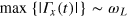 (where
  ), i.e. the counter-propagating term of the control can not be neglected [20, 22]. To fulfill this condition beyond the RWA and to approximate a two-level spin system of
  and
and  , we apply a magnetic field B0 = 1017.3 G (101.73 mT) and set the working transition frequency
  MHz (figure 1(a)). B0 is aligned along the NV crystal axis in order to suppress mixing between the
  and
and  states.

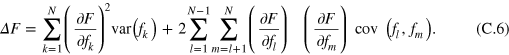
Figure 1. (a) Energy of the  states of the NV centre as a function of the applied static magnetic field B0.
  MHz is the frequency of the transition we used in our experiments. (b) Schematic representation of the pulse sequences for the density matrix tomography. At the beginning we apply a laser pulse to polarize the NV in
  and at the end again to read out the state of the electron spin. The polarization is followed by the optimized π-pulse (CRAB-π, top) or
  -pulse (CRAB-
 , bottom). The tomography is performed by applying
  -pulses along the x- and y-axis of the rotating frame. (c) Rabi frequency as a function of the amplitude of the AWG signal. The circles denote the region where harmonic behaviour is observed as shown in the lower right inset. The red line is a linear fit, its dashed part shows the region where the spin dynamics is anharmonic. The upper left inset shows a typical signal in this region. We chose the MW amplitude which corresponds to the Rabi frequency of
  MHz.
MHz.
Download figure:
Standard image High-resolution image3. Experiments
We begin by measuring Rabi oscillations at different MW amplitudes and observe the spin dynamics (figure 1(c)). When the driving field  the system is in the RWA regime and a nice harmonic signal is obtained (figure 1(c), lower right inset). However, when
  the signal becomes anharmonic as shown in figure 1(c) (upper left inset) and the precise control over the spin rotations is not trivial. Moreover, often the spin is not flipped within certain time as it can be seen from the upper left inset of figure 1(c), where the normalized fluorescence does not drop to zero and the
  state is not reached.
To perform a desired transformation of the spin state  , which follows the Schrödinger equation,
 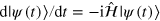 (assuming ℏ = 1), we optimally engineer the time dependence of the control
  , such that at the final time T the state fidelity between the final spin state
  and the target
  is maximized (see also appendix

with  and
and  being respectively the target state and the state expected after the CRAB pulse. Here, we used CRAB controls to implement the two most important single qubit rotations: flipping the qubit (π pulse) and creating a superposition between the qubit states (
 pulse). The experimental realization of these rotations is shown schematically in figure 1(b) while figure 2 shows the calculated trajectories of the spin during the CRAB-π and −π/2 pulses.

Figure 2. (left) The trajectory of the spin magnetization (blue curve) during the application of the CRAB-π pulse. The initial state is  (red-dashed arrow) and the target state is
  (red-solid arrow). (right) After the CRAB-
 , the spin magnetization lays in the
  plane of the lab frame, parallel to the x-axis. Then, it rotates around the z-axis with an angular velocity
  (Larmor frequency), acquiring a phase
  .
.
Download figure:
Standard image High-resolution imageWe set the pulse lengths  ns and
  ns, shorter than
 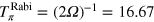 ns and
 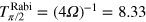 , where
  MHz is the extrapolated Rabi frequency. It is important to note that the latter cannot be used for qubit rotations due to the breakdown of the RWA (see figure 1). The shortest possible pulse length for the π pulse is given by the bang–bang condition
 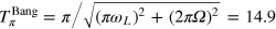 ns [24]. We were not able to approach closer to this limit due to the limited bandwidth and gain curve of the amplifier (refer to appendix
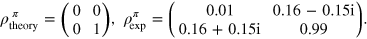
We performed a density matrix tomography in order to determine the quality of the optimized pulses. Both off-diagonal elements have been measured by applying a low power ( MHz)
MHz)  pulse along the x- and y-axis of the rotating frame, followed by a laser pulse for read out (see figure 1(b)). To measure the diagonal elements the MW pulses have been omitted. After the CRAB-π pulse, the theoretically expected and the experimentally measured density matrices are
After the application of optimized CRAB- pulse, we expect
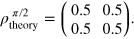
This is the state of the system expected directly after the MW pulse. However, due to limited time resolution of our apparatus, the measurement can be performed only after some dead time. We set this time to  ns during which the spin rotates in the
  plane of the lab frame and acquires a phase
  (see figure 2, right). The density matrix after
  is then
From the tomography, we obtain
The expected fidelities of the CRAB pulses are  and
and  , whilst from the experiment we obtain
 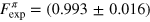 and
and 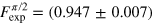 . We find an excellent agreement between the theoretical prediction and the experimental result. The theoretical values are lower than 1 due to the constrains set on the pulse duration. If the pulse length is increased, even higher numerical fidelities can be achieved [25]. The deviation from the prediction can be explained by distortion of the pulse shape, mainly due to the limited bandwidth of the MW amplifier and measurement error (see appendix
The pulses we have developed in this study are important not only for quantum information processing, but also for most of the pulsed nuclear magnetic resonance (NMR) and electron spin resonance (ESR) experiments. They performed the desired spin rotations (π or  as we demonstrate below) up to a global phase factor no matter what the initial states is, although they were optimized for a
  starting state. One of the most important NMR (and ESR) pulse sequences consists of a single
  pulse, where the spin magnetization is rotated from the z-axis to the
  plane in the rotating frame. The spin then precesses and can be detected by the NMR detector thus giving a free induction decay (FID) signal. The Fourier transform of the latter is the spectrum of the sample [26, 27]. This experiment has been already implemented using NV and can be applied for detecting dc magnetic fields [28–30]. Here, we show that we can perform it both in the lab and in the rotating frame by using both CRAB and conventional rectangular pulses. The main difference here compared to previously reported studies, e.g. [30–32], is that we can perform these experiments beyond the RWA.
All sequences begin with a laser pulse for polarising the NV (figure 3(a)). Then we apply a CRAB- pulse, which aligns the spin magnetization along the x-axis of the lab frame. After a free evolution time τ we apply another CRAB-
 pulse to rotate the spin back to the z-axis and we then read out the spin state. The signal oscillates with the Larmor frequency
  (figure 3(a), see also figure 2, right). Here, we measure the signal in the laboratory frame. Now, if we replace the second CRAB-
 pulse with a low power rectangular
  pulse (here
  MHz and
  MHz) and keep its phase fixed for all τ (equivalent to having the B1 parallel to y), again the FID signal oscillates with
  (figure 3(b), blue curve). However, if we set the phase of the second pulse to
  , we can 'follow' the magnetization in the equatorial plane of the Bloch sphere (figure 2, right) and the measurement is performed in the rotating frame and the oscillations at
  disappear (figure 3(b), red markers).
Figure 3. Free induction decays. (a) FID measured by using two CRAB- pulses. The inset shows the first 160 ns of the signal (markers) and the calculated fidelity with respect to the
  state (red solid line, see also text). (b) A combination of a CRAB-
 pulse and a low power
  pulse, where the phase of the latter is fixed for all values of τ (blue curve) and adjusted as
  (red markers), see also the main text. The oscillations with ≈ 2 MHz come from a weakly coupled 13C. (c) FID measured by using low power MW pulses (within RWA), where the phase of the second
  pulse is not in phase with the first pulse (blue markers). If both pulses are kept in phase then the experiment is performed in the rotating frame (red markers). The solid lines are fits to the data. The decay time here is shorter than in the above experiments because the sample is different.
Download figure:
Standard image High-resolution imageThe same experiment can be performed using two rectangular pulses with low MW amplitude (within the RWA) where again the phase of the second pulse is kept constant. In this case the experiment is run in the laboratory frame and the FID again oscillates with the Larmor frequency (figure 3(c), blue markers). If the phase of the MW is not the same for different τ, then we obtain the typical FID in the rotating frame as shown in figure 3(c) (red markers).
Another important sequence is the Hahn echo [33], which has found wide application in NMR and ESR. It is the basis of all dynamical decoupling techniques since all static inhomogeneous shifts (and fluctuations on the time scale of the coherence time T2) are effectively canceled out [26]. It has been implemented with NV [6] and also for NV based ac magnetometry [7, 9]. The Hahn echo pulse sequence is depicted in figure 4(b). After a CRAB- pulse and a free evolution time τ0 a CRAB-π pulse is applied. After a time τ the spin state is rotated to the z-axis by a CRAB-
 pulse and then it is read out by a laser pulse. The spin signal oscillates with the Larmor frequency of the NV transition (in this case
  MHz) as shown in figure 4(a) since the experiment is performed in the lab frame. If we use rectangular pulses in the rotating frame we obtain the envelope of the echo without the oscillations at
  (figure 4(c), red markers). However, we can again 'switch' to the lab frame by adjusting the phase ϕ of the last MW pulse (figure 4(c), blue curve). ESR experiments in the lab frame with low power MW pulses have been already reported [34, 35], but the 'switching' between the two frames in the strong driving regime has not been yet demonstrated. These results demonstrate that we can perform 'textbook' magnetic resonance experiments using the optimally designed pulses.

Figure 4. (a) Hahn echo measured with CRAB-pulses. The signal oscillates with the Larmor frequency (in this case  MHz and the extrapolated Rabi frequency
  MHz), as shown in the three insets. (b) CRAB-Hahn echo pulse sequence. (c) Hahn echo signal obtained with rectangular pulses in RWA when the first MW pulse is not kept in phase with the last two pulses (blue curve) The signal again oscillates with (in this case)
  MHz. The same experiment, here all pulses are kept in phase (red markers). The solid red line is a Gaussian fit to the data. (d) Hahn echo pulse sequence with rectangular pulses where the phase ϕ of the pulses is properly adjusted. (See text for more details.)
Download figure:
Standard image High-resolution image4. Conclusion
In summary, we have developed a novel technique based on optimal control for precise spin qubit rotations in the ultra fast driving regime where standard pulses are not applicable. We design our qubit transformations by using the quantum optimization algorithm CRAB and find an excellent agreement with the experimental implementation. Moreover, we show even when the RWA breaks down the pulses developed here can be used for magnetic resonance experiments. Additionally we demonstrate on demand 'switching' between the rotating and the lab frame, using both CRAB and conventional (low power) pulses. This provides a precise control over the spin evolution and can be easily transferred to any other two level system, e.g. trapped atoms, trapped ions, quantum dots or superconducting qubits. Our results can find wide application in quantum computation and broadband magnetometry.
Acknowledgements
We thank Florian Dolde for the experimental support. This work is supported by EU STREP Project DIAMANT, SIQS, DIADEMS, DFG (SPP 1601/1, SFB TR21) and BMBF (QUOREP). Numerical optimization were performed on the bwGRiD (http://www.bw-grid.de).
Appendix A.: CRAB microwave control
In this section we shortly review the theoretical background of the CRAB method in the context of our current work, and furthermore describe the optimization procedures and the numerical results.
We recall the ground state Hamiltonian of the single electron NV spin in the presence of a single MW control  , as discussed in the manuscript

The CRAB method designs the control  by correcting an initial guess
  with an optimized continuous function g(t), following
  [3, 4]. We use here a simple constant initial guess
  . Following [4], the correcting function g(t) is expanded into a Fourier-like basis function

where N denotes a number of basis expansion having N-randomized discrete frequencies. It is noteworthy to state that the range of frequencies  directly corresponds to the real bandwidth of the apparatus. Therefore, we can pre-set in advance the frequency range for numerical optimization to meet the experimental limitations, e.g. the amplifierʼs or arbitrary waveform generatorʼs working bandwidth. The additional function
  , is used to impose the control boundary such that
  at the initial time t = 0, and the final time T. Here, we choose the bounding function
 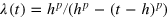 , where
  . Using this function we can also qualitatively vary the rising and falling times of the MW control by adjusting the even-numbered parameter p.
Our optimization objective is to find the set of CRAB parameters { }, which minimizes the figure of merit,
 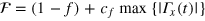 , where the quantity
 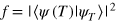 is the fidelity of the final state
  , against the desired state
  . A dimensionless parameter cf
is incorporated in the figure of merit to limit the control amplitude during optimization. We employ the direct search simplex (Nelder–Mead) algorithm to find the optimal CRAB parameters.
. A dimensionless parameter cf
is incorporated in the figure of merit to limit the control amplitude during optimization. We employ the direct search simplex (Nelder–Mead) algorithm to find the optimal CRAB parameters.
The numerical optimization is initiated by setting some parameters obtained from the experimental preparations and apparatus calibrations: the measured Larmor transition  , the maximum control amplitude
 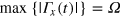 , and the CRAB frequency range. The control time is fixed (the same as the desired rotation time) to be faster than the extrapolated rotation time if the RWA would be valid, e.g. for the spin
  -rotation we have
  1/2Ω−1, where Ω is the extrapolated Rabi frequency (see figure 1(c)). However, the
  -rotation time in our case is limited by the minimum time of the theoretically proposed optimal bang–bang control,
 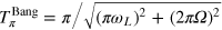 , where the control
  takes only a constant value of
  for a certain time interval [24]. To obtain the optimized pulse for one target rotation, we do the following steps:
- (1)Perform the parallel simplex search algorithm with an S number of random initial values of the CRAB parameters for j small positive real numbers of
 , and k positive small integers , typically and .
 - (2)Obtain from step 1, sets of CRAB parameters, than construct numbers of control pulses .
- (3)Investigate the numerical values of and for each pulse, and pick the best one out of pulses which satisfies and . The preset quantities κf
and are the numerical infidelity and the maximum control amplitude, respectively. If the best pulse can not be obtained, return to step 1 with different values of and increase .


The actual numerical calculations were carried out on the bwGRiD cluster where we utilized its multi-nodes multi-cores (eight cores per node) computational features to run the parallel Nelder–Mead searches that corresponds to various experimental parameters and random initial values. To find a single parallel sample in one-core, i. e. one set of CRAB optimized parameters, the typical computational time required to meet the experimentally acceptable fidelity is approximately less than 30 min. This allows one to perform a single optimization run in just a decent commercial personal computer. Hence, it is feasible in the future to apply our numerical CRAB optimization in standard close-loop control system involving directly the control apparatuses. For both cases of  -rotation and
  -rotation we set the parameters as the following: N = 5, S = 30,
  MHz, and
  MHz. We present the best obtained CRAB parameters for each rotation in table A.1
, while the corresponding MW pulses are shown in figure B.1.
MHz. We present the best obtained CRAB parameters for each rotation in table A.1
, while the corresponding MW pulses are shown in figure B.1.

Figure B.1. Pulse Shapes. (a) Oscilloscope measurement of the signal after the diamond sample with the standard sinusoidal microwave after 100 ns delay to measure Rabi oscillations for the state tomography. (b) CRAB-π pulse (blue) in comparison to numerical pulse (red). (c) CRAB-π/2 pulse (blue) in comparison to numerical pulse (red).
Download figure:
Standard image High-resolution imageTable A.1.
The optimal CRAB parameters obtained via the Nelder–Mead simplex algorithm for π- and  -rotations. The corresponding MW-CRAB pulses are shown in figure B.1.
| π-rotation |
 -rotation -rotation |
||||
|---|---|---|---|---|---|
| T = 15.4071 ns, p = 60, cf = 0.35 | T = 7.7036 ns, p = 38, cf = 0.23 | ||||
| an | bn | ωn (GHz) | an | bn | ωn (GHz) |

|

|

|

|

|

|

|

|

|

|

|

|

|

|

|

|

|

|

|

|

|

|

|

|

|

|

|

|

|

|
Appendix B.: Experimental setup and pulse shapes
The pulses optimized by the CRAB algorithm is a superposition of ten periodic functions. In the experiment, these pulses are synthesized directly by an arbitrary waveform generator (AWG, Tektronix AWG7122C) with a sampling rate of 24 GS s−1 and then sent to an amplifier (Mini-Circuits, ZHL-42W-SMA). The pulse shapes measured via an oscilloscope (Tektronix, TDS6804B) are displayed in figure B.1.
Optical measurements were obtained via a self-made confocal microscope, the AWG triggered both the acousto-optic modulator for laser pulse control and the photon-count card (FastComtec P7887).
Appendix C.: State tomography
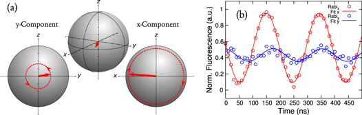
In order to determine the fidelity of the final state in respect to the target state we performed a state tomography. For this purpose we evaluated all three components of the Bloch vector. The z-component is measured directly from the fluorescence level. The x- and y-components have to be projected into the measurable z-component. This is done by applying a MW with different phases and measure Rabi oscillations or in other words: rotate the Bloch vector around the x-axis to determine the y-component and vice versa, as shown in figure C.1.
Figure C.1. State tomography. (a) The state is characterized by performing Rabi oscillations by rotating the spin around the x- and y-axis. The z-component can be observed by measurement without application of a microwave. With the amplitude and the z-component the x- and y-component can be calculated simply using the Pythagorean theorem. (b) Measurement data of the state tomography after the CRAB- -pulse.
Download figure:
Standard image High-resolution image
The density matrix of a single qubit can be written as

In this definition,  and z have values between −1 and 1. The first point of the measurements
  and
and  , where no MW was applied, can be understood as the z-component. The three components of the Bloch vector are calculated following


where  and z are the three components of the Bloch vector and
  are the amplitudes of the Rabi oscillations rotating around the y, x-axis respectively. In formula C.3 and C.4, values for x and y were set to 0 if the uncertainty was greater than the actual value. Another possibility to obtain the x- and y-component is to calculate
  and
and  respectively.
To normalize the data we performed an additional, bare Rabi measurement. The normalization is done by  , where A is the amplitude and y0 is the offset of the normalization measurement.
In order to calculate the fidelity between the experimental state ρ and the target state  the definition for pure states is used:
 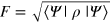 which in this case is equivalent to the general definition
 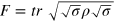 [23].
[23].
Due to experimental limitations we had to wait for 100 ns between the CRAB-pulse and the Rabi measurement, hence the target state after the time evolution on the  plane becomes

with the Pauli matrix σz and the Larmor frequency  . For the error calculation of the fidelity the noise of the Poisson distributed photon collection and fitting errors were taken into account. The error was determined by using the general law of error propagation [36]