


Abstract
A new regime of relativistic high-order harmonic generation has been discovered (Pirozhkov 2012 Phys. Rev. Lett. 108 135004). Multi-terawatt relativistic-irradiance (>1018 W cm−2) femtosecond (∼30–50 fs) lasers focused to underdense (few × 1019 cm−3) plasma formed in gas jet targets produce comb-like spectra with hundreds of even and odd harmonic orders reaching the photon energy of 360 eV, including the 'water window' spectral range. Harmonics are generated either by linearly or circularly polarized pulses from the J-KAREN (KPSI, JAEA) and Astra Gemini (CLF, RAL, UK) lasers. The photon number scalability has been demonstrated with a 120 TW laser, producing 40 μJ sr−1 per harmonic at 120 eV. The experimental results are explained using particle-in-cell simulations and catastrophe theory. A new mechanism of harmonic generation by sharp, structurally stable, oscillating electron spikes at the joint of the boundaries of the wake and bow waves excited by a laser pulse is introduced. In this paper, detailed descriptions of the experiments, simulations and model are provided and new features are shown, including data obtained with a two-channel spectrograph, harmonic generation by circularly polarized laser pulses and angular distribution.
General Scientific Summary
Introduction and background. Bright coherent x-rays are indispensable for fundamental research and numerous applications in bio- and nanotechnology, chemistry, etc. Now such x-rays are obtained with free electron lasers. Relativistically intense laser-matter interaction producing bright high-order harmonics is an attractive alternative.
Main results. We discovered a new regime of high-order harmonic generation by multi-terawatt femtosecond lasers focused to micrometre spots in supersonic gas jets, figure 1(a). The focused laser irradiance exceeds 1018 W cm−2 rendering the interaction relativistically intense. Using either linearly or circularly polarized laser pulses, we observed coherent x-rays emitted from the gas jet. The obtained spectrum is comb-like, figure 1(b), with hundreds of even and odd harmonic orders reaching the 'water window', up to the photon energy of 360 eV. We found that the maximum photon energy grows as the laser amplitude cubed, while the photon number scales faster than linearly with the laser power. With a 120 TW laser, we obtained 4 × 10⁹ photons (90 nJ pulse energy) in a single harmonic at 120 eV. Using Particle-In-Cell simulations and mathematical catastrophe theory, we explained our experiments by a new high-order harmonic generation mechanism: a tightly focused laser in plasma forms structurally stable electron spikes which coherently emit high-order harmonics, figure 1(c).
Wider implications. Our work paves the way to a bright coherent keV x-ray source based on table-top lasers and accessible, self-replenishable, and debris-free gas jet targets. Such a source will be crucial for pumping, probing, imaging of microscopic objects and for attosecond science.
Figure. New regime of high-order harmonic generation by relativistic laser focused into gas jet target. (a) Experimental setup. (b) Typical single-shot raw data. (c) 3D particle-in-cell simulation demonstrating electron density spike and location of high-order harmonics source. Download figure:
Export citation and abstract BibTeX RIS

Content from this work may be used under the terms of the Creative Commons Attribution 3.0 licence. Any further distribution of this work must maintain attribution to the author(s) and the title of the work, journal citation and DOI.
General Scientific Summary
Introduction and background. Bright coherent x-rays are indispensable for fundamental research and numerous applications in bio- and nanotechnology, chemistry, etc. Now such x-rays are obtained with free electron lasers. Relativistically intense laser-matter interaction producing bright high-order harmonics is an attractive alternative.
Main results. We discovered a new regime of high-order harmonic generation by multi-terawatt femtosecond lasers focused to micrometre spots in supersonic gas jets, figure 1(a). The focused laser irradiance exceeds 1018 W cm−2 rendering the interaction relativistically intense. Using either linearly or circularly polarized laser pulses, we observed coherent x-rays emitted from the gas jet. The obtained spectrum is comb-like, figure 1(b), with hundreds of even and odd harmonic orders reaching the 'water window', up to the photon energy of 360 eV. We found that the maximum photon energy grows as the laser amplitude cubed, while the photon number scales faster than linearly with the laser power. With a 120 TW laser, we obtained 4 × 10⁹ photons (90 nJ pulse energy) in a single harmonic at 120 eV. Using Particle-In-Cell simulations and mathematical catastrophe theory, we explained our experiments by a new high-order harmonic generation mechanism: a tightly focused laser in plasma forms structurally stable electron spikes which coherently emit high-order harmonics, figure 1(c).
Wider implications. Our work paves the way to a bright coherent keV x-ray source based on table-top lasers and accessible, self-replenishable, and debris-free gas jet targets. Such a source will be crucial for pumping, probing, imaging of microscopic objects and for attosecond science.
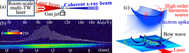 Figure. New regime of high-order harmonic generation by relativistic laser focused into gas jet target. (a) Experimental setup. (b) Typical single-shot raw data. (c) 3D particle-in-cell simulation demonstrating electron density spike and location of high-order harmonics source.
1. Introduction
High-order harmonic generation is one of the most fundamental processes of nonlinear optics. The coherency of high-frequency radiation associated with high-order harmonics is necessary for the tightest focusability and generation of ultrashort pulses required for applications. Numerous nonlinearities produce high-order harmonics in various laser–matter interaction regimes. At irradiances of the order of 1018 W cm−2 and higher, corresponding to relativistic plasma dynamics [1, 2], several regimes of high order harmonics generation are known, including laser–solid target interaction [3–8], harmonics generation in a plasma channel [9], and the second harmonic from electro-optic shocks [10, 11]. Nonlinear Thomson scattering [12] by plasma electrons [13–17] and electron beams [18, 19] also produces harmonic spectra. At typical irradiances from ∼1013 to 1015 W cm−2 harmonics are generated in atomic [20] or molecular [21] gases or in cold ablation plumes [22] via the nonlinearity of ionizing matter [23, 24]; a review of this process and related issues can be found in [25]. Recently [26] we discovered a new high-order harmonic generation regime in relativistic laser plasma, explained by a new mechanism based on catastrophe theory [27, 28].
The two most important parameters determining the relativistic laser–plasma interaction are the dimensionless laser pulse amplitude a0 = eE0/mecω0 and ratio ne/ncr of the electron density ne to the critical density ncr = meω02/4πe2 = π/reλ02 ≈ 1.1 × 1021 cm−3 (μm/λ0)2. Here e and me are the electron charge and mass, c is the speed of light in vacuum, re = e2/mec2 ≈ 2.8 × 10⁻¹³ cm is the classical electron radius, and λ0, ω0, and E0 are the laser wavelength, angular frequency, and peak electric field, respectively. The laser irradiance in terms of the dimensionless amplitude is I0L ≈ a02 × 1.37 × 1018 W cm−2 × (μm/λ0)2 for linear and I0C = 2I0L for circular polarizations.
In this paper we consider a relativistically strong laser pulse, a0 ⩾ 1, and underdense plasma, ne/ncr ∼ 0.01 (see the details in the setup description below). Under these conditions plasma is essentially collisionless [29]. Propagating through the plasma, the laser pulse undergoes relativistic self-focusing [30–34] when its power P0 exceeds the critical power [32, 34] PSF:
Under our conditions, the typical values are ne ∼ 1019 cm−3, and λ ∼ 1 μm, thus giving PSF ∼ 2 TW. For mid-infrared lasers and high-density gas jets (ne ∼ 1020 cm−3) the critical power for self-focusing can be smaller than ∼ 100 GW. Due to self-focusing, the laser pulse acquires a much higher amplitude, which can be estimated using the stationary focusing condition [35]
while the focal spot diameter is
where ωpe = (4π ne e2/me)1/2 is the Langmuir frequency.
In the course of the relativistic laser–plasma interaction, nonlinear plasma waves are generated. The bow wave [36] is generated by the electrons expelled in the transverse direction. The bow wave formation condition, dSF < 4aSF1/2 c/ωpe, is satisfied during the stationary self-focusing, equation (3). The wake wave [37], emerging from the longitudinal electron oscillations, produces a moving potential, which is the basis of the laser wake-field accelerator (LWFA) concept [38, 39]. The electrons, spontaneously injected into and accelerated by the wake wave and oscillating in the plasma channel, can emit betatron x-ray radiation [40–42]. Nearly-breaking nonlinear wake waves act as partially reflective relativistic flying mirrors [43–47] for counter-propagating electromagnetic radiation. The flying mirror upshifts the frequency and shortens the duration of a reflected pulse due to the double Doppler effect, and also focuses the reflected pulse due to the close-to-parabolic mirror surface [48, 49].
In this paper we describe new features of the high-order harmonic generation regime in underdense relativistic laser plasma, first described in [26], including data obtained with a two-channel spectrograph, harmonic generation by circularly polarized laser pulses, spatial coherence and angular distribution. We compare the properties of the harmonics in the new generation regime with the previously known scenarios and show that several advantages make the new regime a possible candidate for a next-generation compact coherent x-ray source.
The paper is organized as follows. In section 2 we describe the experimental setup, followed by the experimental results in section 3. Section 4 contains a comparison of the observed harmonics with the previously suggested mechanisms, and a discussion about possible harmonics origin. Section 5 contains simulation results and their analysis, followed by a description of the new harmonics generation mechanism in section 6, a catastrophe theory based model in section 7, and simplified scaling in section 8. Section 9 contains our conclusions.
2. Experimental setup
We have performed experiments with the J-KAREN laser in KPSI, JAEA, Japan [50] and the Astra Gemini laser in the CLF, RAL, UK [51]. The laser parameters used in these experiments are listed in table 1. The J-KAREN laser has the pulse energy EL = 0.4 J, peak power P0 ≈ 9 TW, and central wavelength λ0 = 820 nm. The pulse duration measured with our transient grating frequency resolved optical gating (TG FROG) [52] is typically τ ≈ 27 fs (full width at half maximum, FWHM), with respect to power. The laser pulses are focused by an f/9 off-axis parabolic mirror down to the spot size of ∼10–12 μm FWHM and ∼20–30 μm at 1/e2 intensity level measured by imaging the spot with magnification onto a charge-coupled device (CCD) using a laser pulse sufficiently attenuated with wedges. The derived peak irradiance in vacuum is I0 ≈ 4 × 10¹⁸ W cm−2. For the Astra Gemini laser, the pulse energy EL is up to 10 J, P0 ranges from 60–170 TW, central wavelength λ0 = 804 nm, and typical duration τ ≈ 54 fs (FWHM) measured with spectral phase interferometry for direct electric field reconstruction (SPIDER). With an f/20 off-axis parabolic mirror, the typical focal spot size is 25 μm × 40 μm (FWHM) and ∼40 μm × 80 μm at 1/e2; these spot sizes are estimated from far field images of leakage through dielectric mirrors during the full-power shots. The derived peak irradiance in vacuum ranges from 2 × 10¹⁸–5 × 10¹⁸ W cm−2.
Table 1. Parameters of lasers used in the experiments: pulse energy EL, peak power P0, central wavelength λ0, FWHM pulse duration τ, focusing f-number, FWHM and 1/e2 spot sizes, peak irradiance and dimensionless amplitude in vacuum I0 and a0, and estimated dimensionless amplitude after self-focusing aSF, equation (2). The peak power P0 and irradiance I0 are estimated from the temporal pulse shape s(t) and focal spot fluence distribution u(x, y) measured at reduced laser power, i.e. EL = P0∫s(t)dt and EL = I0∫u(x, y)dxdy∫s(t)dt, where u(x, y) and s(t) are normalized to their maximum values, i.e. max[u(x, y)] = 1 and max[s(t)] = 1.
| Laser | EL (J) | P0 (TW) | τ (fs) | λ0 (nm) | f-number | Spot FWHM [1/e2] (μm) | I0 (W cm−2) | a0 | aSF, equation (2) |
|---|---|---|---|---|---|---|---|---|---|
| J-KAREN | 0.4 | 9 | 27 | 820 | f/9 | 10 [20] | 4 × 10¹⁸ | 1.4 | 5–8 |
| Astra Gemini | 3–10 | 60–170 | 54 | 804 | f/20 | 25 × 40 [40 × 80] | 2 × 10¹⁸–5 × 10¹⁸ | 1–1.5 | 12–16 |
The experimental setups are schematically shown in figure 1. The J-KAREN laser pulses have been focused into a supersonic high-purity helium gas jet streamed from a conical nozzle with the orifice diameter of 1 mm and calculated Mach number of M = 3.3 at a distance of 1 mm from the nozzle orifice. In the experiment with the higher-energy Astra Gemini laser, a conical nozzle with a smaller diameter 0.5 mm orifice with M = 2.0 has been used to decrease the energy of the accelerated electrons (by decreasing the acceleration length) and thus reduce the noise generated by hard x-ray photons. We noticed nozzle degradation after shots performed at the 1 mm distance between the focus and the nozzle orifice and, therefore, increased this distance to 1.5 mm. The gas density distribution has been characterized with interferometry using Ar gas, figure 2 (inset). The Ar gas clusterization does not significantly affect the density measurement because for Hagena's parameter [53] values of Γ* < 7 × 10⁴, the dryness is nearly at unity with an accuracy of a few percent [54] and, thus, the Ar density is close to the He density. We have not observed shocks at the gas jet–ambient gas interface. The electron density of the helium plasma is calculated to be twice the atomic density in the gas jet, because the laser irradiance significantly exceeds the threshold of the barrier suppression double ionization of helium [55]. Typical distributions of plasma density are shown in figure 2. The bright harmonic spectra are observed when the maximum electron density ranges from 1.7 × 10¹⁹–7 × 1019 cm−3, which corresponds to 0.01 ⪅ ne/ncr ⪅ 0.04 for λ0 = 820 nm. Weaker spectra are detectable for densities down to 1.5 × 1019 cm−3 and up to ∼1020 cm−3. The density gradient varies by a factor of five, from 2 × 10²⁰–11 × 1020 cm−4. The parameters of the gas jet targets are listed in table 2.

Figure 1. Experimental setup schematics for relativistic high-order harmonic generation in gas jet targets, the experiments with the J-KAREN (a) and Astra Gemini (b) lasers. The multi-TW femtosecond lasers irradiating He gas jets generate XUV and soft x-ray high-order harmonics detected with the grazing-incidence flat-field spectrographs, dashed rectangles. The spectrograph in the experiment with the Astra Gemini laser has two channels separated by 0.53°. The electrons accelerated by the lasers are deflected from the spectrographs by the permanent magnets and analysed with the electron spectrometers, dotted rectangles.
Download figure:
Standard image High-resolution image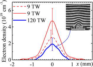
Figure 2. Typical plasma density profiles used in the experiments. The inset shows an example of an interferometric image of the Ar gas jet used for measurement of the gas density distribution.
Download figure:
Standard image High-resolution imageTable 2. Parameters of the gas jet targets: nozzle orifice diameter d, distance from the laser axis to the nozzle orifice h, calculated Mach number M, ambient pressure PVac, backing pressure Pb, peak electron density ne,max, density gradient dne/dx.
| Laser | Nozzle type | d, mm | h, mm | M | PVac, Pa | Pb, MPa | ne,max, 1019 cm−3 | dne/dx, 1020 cm−4 |
|---|---|---|---|---|---|---|---|---|
| J-KAREN | Conical | 1 | 1 | 3.3 | <10−2 | 0.6–3.1 | 1.5–9.6 | 2 to 11 |
| Astra Gemini | Conical | 0.5 | 1.5 | 2.0 | <10−2 | 3.1–9.9 | 1.5–4.6 | 2 to 6 |
In our experiments the peak power in vacuum for both lasers significantly exceeds the critical power of the relativistic self-focusing, equation (1). Thus, during propagation in plasma the laser pulses self-focus, acquiring much higher irradiances than in vacuum. We note that the density gradient influencing the laser–target interaction [6, 8, 56] and the focusing optics f-number can be used for the optimisation of channel formation, laser pulse propagation and self-focusing [57–59]. As is typical for this parameter regime, we observe electron acceleration up to a few hundred MeV. To reduce the noise caused by bremsstrahlung x-rays, these electrons are deflected from the measurement direction by permanent magnets, and directed to the phosphor screens of the electron spectrometers.
The extreme ultraviolet (XUV) and soft x-ray harmonics have been observed in the forward direction with grazing-incidence flat-field spectrographs comprising a gold-coated collecting mirror, spherical varied-linespace grating, and back-illuminated CCD shielded by optical blocking filters. The parameters of the spectrographs are summarized in table 3. The observable spectral regions are 80–250 eV or 110–360 eV with the J-KAREN and 110 to 200 eV with the Astra Gemini lasers. The spectrograph used with the Astra Gemini laser consists of two channels with observation angles of α0 ≈ 0° (forward direction) and α0 + 0.53° (in the laser polarization plane for linear polarization); the spectrograph is operated in the 2nd and 3rd diffraction orders in order to reduce the scattered light arising from the zeroth order. The throughputs of the spectrographs, defined as products of the collecting mirror reflectivity, filter transmission, grating efficiency, and CCD quantum efficiency, are shown in figure 3(a). The mirror reflectivities and filter transmissions are calculated using the atomic scattering factors [60–62]. Measurements by the manufacturer at several wavelengths are in good agreement with the calculations, figure 3(b). The diffraction efficiencies at the incidence angles and diffraction orders used in these experiments have been measured using synchrotron radiation [63, 64]; comparison of the harmonic spectra obtained from the second and third diffraction orders (see later, in figure 6(c)), suggests that the diffraction efficiencies are valid with a relative accuracy of better than several percent. Quantum efficiency data and gain are provided by the CCD manufacturers.
Table 3. Parameters of the grazing-incidence flat-field spectrographs.
| Spectrograph [46, 79] used with the J-KAREN laser | Two-channel spectrograph [80] used with the Astra Gemini laser | |
|---|---|---|
| Collecting mirror | Gold-coated toroidal mirror | Gold-coated ellipsoidal tapered mirrors |
| Incidence angle | 88° | 88.5° (on-axis), 86.9° (0.53° off-axis) |
| Acceptance angle | 3.0 × 10⁻⁵ sr | 3.0 × 10⁻⁶ sr and 7.5 × 10⁻⁶ sr |
| Slit | 200 μm slit | No slit |
| Optical blocking filters | Two multilayer Mo/C filters [81] or two Pd filters | One Ag filter on CH substrate |
| Thickness | Mo/C: 0.16 μm, Pd: (0.20 ± 0.02) μm | Ag: (0.20 ± 0.02) μm, CH: 0.1 μm |
| Spectral range, nm | 5–15 nm or 3.5–11 nm | 3–11 nm |
| Spectral range, Ev | 80–250 eV or 110–360 eV | 110–200 eV |
| Diffraction grating | Spherical flat-field grating | Spherical flat-field grating |
| Average groove density | 1200 lines/mm | 1200 lines/mm |
| Incidence angle | 87° | 84.6° |
| Diffraction order | m = 1 | m = 2 and m = 3 |
| CCD | Back-illuminated CCD | Back-illuminated CCD |
| Gain | 0.315 counts/electron energy per electron-hole pair 3.65 eV | 0.143 counts/electron energy per electron-hole pair 3.65 eV |
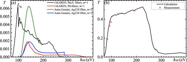
Figure 3. (a) Throughputs of the spectrographs; the curves are shown up to the limits determined by the CCD edges. LSi denotes the Si absorption edge of known silicon contamination. (b) Comparison of calculated and measured transmission of one of the Mo/C filters.
Download figure:
Standard image High-resolution imageThe wavelength calibration of both spectrographs is carefully performed using the spectra of Ar and Ne plasmas excited in-place by the same laser. Due to the finite resolving power of the spectrographs and the few hundred μm size of the emitting plasma region, the spectral lines of Ar and Ne ions are two to four pixels wide on the CCDs. Using many spectral lines, and determining line centres by multi-peak Gaussian fitting, we achieved sub-pixel calibration accuracy. To illustrate the method, the calibration of the spectrograph used with the Astra Gemini laser is shown in figure 4. In experiments with both setups (for J-KAREN and Astra Gemini lasers), the relative calibration error estimated from spectral line wavelength errors and difference between shots is δλ/λ ∼ a few × 10−4. Additional confidence in the spectral calibration accuracy follows from the correct wavelengths of silicon and carbon absorption edges visible in the data (e.g. figure 5 at 100 eV and figure 13 at 284 eV) and identical harmonic structures obtained from the second and third diffraction orders, figure 6(c).
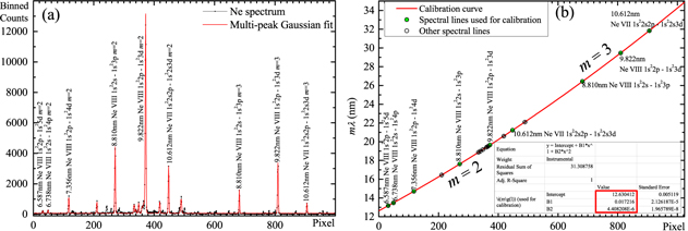
Figure 4. Wavelength calibration of the on-axis channel of the spectrograph used with the Astra Gemini laser. (a) Black dots connected with black line: lineout of Ne spectrum; the Ne plasma from a mixture of He and Ne gases is created by the laser at the same position as in the case of the pure He jet which has been used for the harmonics generation. Red line: multi-peak Gaussian fit, from which precise positions of the selected spectral line centres are found. (b) Calibration curve obtained by the second order polynomial fit of spectral lines shown by the filled circles. The spectral lines not used for the calibration are shown by open circles to confirm the calibration accuracy.
Download figure:
Standard image High-resolution image
Figure 5. A typical harmonic spectrum obtained with the laser power P0 = 9 TW and peak electron density ne = 2.7 × 1019 cm−3. (a) Raw data. (b) The lineouts of two selected six pixel wide regions, dashed brackets in (a), demonstrating harmonic structure with the base frequency ωf = 0.885ω0 denoted by the vertical lines, where ω0 is the laser frequency. The highest distinctly resolved order is nH* = 126, denoted by the circle in (b).
Download figure:
Standard image High-resolution image
Figure 6. Harmonic spectrum obtained with P0 = 120 TW, ne = 1.9 × 1019 cm−3, ωf = 0.537ω0, linear polarization. (a) Raw data. The top and bottom spectra correspond to the 0.53° off-axis and on-axis channels, respectively. The inset shows a magnified portion of the on-axis spectrum, denoted by the white rectangle. The spectrograph operates in the second and third diffraction orders, m; the wavelengths and photon energies for m = 2 and 3 are shown by the blue and green numbers, respectively. (b) Lineout along a narrow (three pixel wide) stripe corresponding to the on-axis channel demonstrating resolved harmonics, dashed bracket in (a). (c) On-axis harmonic spectra from the second (thick blue line) and third (thin green line, multiplied by 1.12) diffraction orders. The harmonic structure and period coincide, while the spectral intensity differs by only 12%, confirming the wavelength calibration and throughput calculation accuracy.
Download figure:
Standard image High-resolution image3. Experimental results
High-frequency radiation with photon energy from ћω = 75–360 eV (corresponding to the full range of the spectrographs used) has been observed in the interaction of laser pulses (either linearly or circularly polarized) with power from P0 = 9–170 TW, and helium gas jets with an estimated maximum electron density from ne = 1.7 × 10¹⁹–7 × 1019 cm−3. The representatives of the variety of observed single-shot spectra are shown in figures 5– 7, 9, 10, 12 and 13. Simultaneously the electrons with broad spectra and energies up to a few hundred MeV have been measured. These electrons exhibit no apparent correlation with the high-frequency radiation properties. At lower plasma densities, higher-energy quasi-monoenergetic electron acceleration can be achieved, however the high-frequency radiation disappears. We also note that only usual thermal plasma emission has been observed in the cases of Xe, Ar, Ne, and CO2 gas jets.

Figure 7. Harmonic spectrum obtained with P0 = 170 TW, ne = 4 × 1019 cm−3, circular polarization. (a) Raw data. The inset shows a magnified portion of the on-axis spectrum, denoted by the white rectangle. (b) Lineout along a narrow (three pixel wide) stripe corresponding to the inset in (a). (c) Fourier transformation of the spectrum in the spectral range from 120–160 eV. The clear narrow peak at 2.33 eV−1 corresponding to ћωf = 0.429 eV shows the spectrum periodicity. (d) Lineout corresponding to the dashed brace in (a) demonstrating harmonics resolved up to the ∼370th order, black circle. (e) Fourier transformation of the spectrum in the spectral range from 140–160 eV shown in (d), the peak almost coincides with the vertical dashed line corresponding to the peak in frame (c), thus confirming the same spectrum periodicity in this spectral region; the black dashed line shows the noise level.
Download figure:
Standard image High-resolution imageThe comb-like spectra comprising odd and even harmonics of similar intensity and shape are generated in the specified broad range of laser and plasma parameters, demonstrating the effect's robustness. This represents the majority of cases observed with the high-resolution spectrograph [65]. The spectra obtained with linearly polarized laser pulses are shown in figure 5 for the laser power of 9 TW, and in figure 6 for 120 TW. The spectrum obtained with the circularly polarized laser pulse is shown in figure 7 for 170 TW. In the case of circular polarization, the harmonic generation typically requires higher laser power or greater plasma density; however, additional experimental data are required to quantify the differences in optimum conditions for linear and circular polarizations.
Thanks to the high quality of the data and high calibration accuracy, several important features of the harmonic spectra are revealed. The base frequency of the spectra, ωf, is downshifted from the laser frequency, ω0. We attribute this to the well-known gradual frequency downshift of a laser pulse propagating in tenuous plasma [1, 39, 66, 67]. When the laser pulse transfers its energy to plasma waves in the adiabatic limit, the photon number is approximately conserved. This leads to the corresponding photon energy decrease, i.e. the frequency red-shift. This carrier frequency downshift of the laser pulse appears in the transmitted laser spectra, figure 8(a), in accordance with the observed base harmonic frequency.

Figure 8. (a) Red solid line, the spectrum of laser pulse transmitted through plasma for the shot when the harmonic spectrum shown in figure 5 is obtained; the blue vertical line corresponds to ωf = 0.885ω0. The dashed line corresponds to the laser pulse spectrum recorded with the same setup, but without plasma. The spectra are corrected for the overall detection system sensitivity. (b) Resolving power of spectrograph used with the J-KAREN laser estimated from widths of spectral lines in the Ne spectrum (circles); the thick line shows the parabolic fit. The thin dotted and solid lines show the resolving power necessary to distinguish individual harmonics at the corresponding wavelength for the base harmonic frequency equal to the laser frequency ω0 and 0.885ω0, respectively. The numbers indicate the maximum resolvable harmonic orders and are limited by the spectrograph's resolving power.
Download figure:
Standard image High-resolution imageAnother feature is a large number of resolved harmonics. For example, harmonics up to nH* ∼ 126th order are clearly distinguishable in figure 5 and up to nH* ∼ 370th in figure 7. In both cases, these numbers are close to the limits determined by the resolving power of the spectrographs. Figure 8(b) shows the resolving power of the spectrograph, which recorded the spectrum shown in figure 5, as estimated from the widths of spectral lines in neon plasma. The spectrograph enables resolving of at most ∼140 harmonics for the downshifted base frequency of ωf = 0.885ω0. As for figure 7, the separation between peaks in the spectrum approaches a two CCD pixels span, i.e. also the resolution limit. Despite this, the spectrum periodicity is clearly visible in the raw data figure 7(a), lineouts (b, d), and Fourier transformations (c, e).
The large number of distinctly resolved harmonic orders nH* together with the gradual frequency downshift allow estimation of the harmonic's emission length δx. During the emission, the relative frequency drift, δω/ω, cannot be larger than (1/2nH*), otherwise the harmonics nH* and nH* + 1 overlap. The relative frequency change is approximately equal to the relative energy change [66, 67], δω/ω ≈ δx/Ldep, where Ldep is the depletion length. Therefore, δx ≈ Ldep/2nH*. We estimate Ldep ∼ 2.7 mm from the 70% energy transmission through the 0.9 mm long plasma, figure 8(a). For the harmonics spectrum shown in figure 5 this gives δx ≦̸ 12 μm, which is the upper bound, since the number of resolved harmonic orders may be limited by the spectrograph resolving power. Here we note that the longitudinal size of the harmonic's source can be much shorter than the emission length.
In the case of linearly polarized laser pulses, in some shots the spectra exhibit deep equidistant modulations, figure 9. There are even cases with the modulation depth approaching 100%. Such modulations are also visible in the case of unresolved or nearly unresolved harmonics, figure 10. The spectra with unresolved harmonics typically contain a larger photon number. These features can be explained by a longer harmonics emission time, during which the greater continuous downshift of the laser frequency leads to the observed harmonic structure blurring. In a total of 90 shots with circularly polarized 50–200 TW pulses, the large-scale spectral modulations have not been observed.

Figure 9. A typical modulated harmonic spectrum with resolved individual harmonics, P0 = 9 TW, ne = 4.7 × 1019 cm−3, ωf = 0.872ω0. (a) Raw data. (b) The lineout of the selected six pixel wide region, the dashed bracket in (a). The vertical lines denote modulation period in the frequency domain Δω = 19ωf.
Download figure:
Standard image High-resolution image
Figure 10. A typical modulated harmonic spectrum with nearly unresolved harmonics, P0 = 9 TW, ne = 4.7 × 1019 cm−3. (a) Raw data. (b) The lineout of the selected seven pixel wide region, the dashed bracket in (a). The modulation period in the frequency domain, Δω = 6.08ωf, is denoted by the solid vertical lines.
Download figure:
Standard image High-resolution imageTwo spectrograph channels observing the harmonics on-axis and 0.53° off-axis, figures 6 and 7, show spectra with similar intensities, figure 11, taking into account the ≈ 2.5-fold difference in acceptance angles determined during calibration using a nearly isotropic neon plasma emission. However, in some shots one of the channels shows a several times greater signal than another. These observations indicate that the angular distribution of the harmonic emission has a characteristic size of several degrees with possible direction fluctuations of the order of a few degrees. The high-resolution 2D particle-in-cell (PIC) simulations performed with the code REMP [68] (see below), suggest that the harmonics are emitted slightly off-axis and for harmonic orders of about a hundred their angular span is ∼3°.

Figure 11. Comparison of total signals recorded with various experimental parameters by the on-axis and off-axis channels, the colour encodes the He backing pressure. In the majority of shots, the signal ratio of the two channels is close to the acceptance angle ratio (slope of the dashed line), although in some shots the signal ratio deviates from the general trend.
Download figure:
Standard image High-resolution imageA remarkable feature of the harmonic spectra is their high brightness, so each of the spectra shown in this paper is the result of a single-shot acquisition. The harmonic pulse energy and photon numbers are conservatively estimated using spectrograph throughputs, figure 3(a). Examples of the spectra in the units of μJ/(eV·sr) are shown in figures 6(c), 12 and 13. These data are obtained within the respective acceptance angles of the spectrographs; thus, without the necessity of assumptions on the angular distribution and spatial beam profile. The photon yield scales favourably with the laser power, as follows from the comparison of the harmonics spectra obtained with the 9 TW and 120 TW laser powers, figure 12.

Figure 12. Comparison of the spectra obtained with the 9 TW and 120 TW lasers. The upper (blue) line corresponds to the 120 TW laser, the same shot as shown in figure 6. The lower 9 TW red line with distinctly resolved harmonics corresponds to the shot shown in figure 5. The upper 9 TW red line corresponds to the shot shown in figure 13.
Download figure:
Standard image High-resolution image
Figure 13. The spectrum within the ʽwater window' spectral region obtained with the 9 TW laser, ne = 4.7 × 1019 cm−3. The signal drops at ∼284 eV due to hydrocarbon contamination of the optics at the carbon K absorption edge, KC. The dashed curve indicates the noise level.
Download figure:
Standard image High-resolution imageAt 120 TW laser power, the harmonic pulse energy and photon number in a unit solid angle reach 40 μJ sr−1 and 2 × 10¹² photons sr−1 in one harmonic at 120 eV. Assuming the 3° angular width derived from the simulations, these amount to 90 nJ pulse energy and 4 × 10⁹ photons.
The spectrograph used with the 9 TW laser has a throughput cut-off at ∼360 eV with the Pd filters, figure 3(a). The harmonic emission extends up to this photon energy, figure 13, thus reaching the 'water window' spectral range enclosed between the K absorption edges of carbon at 284 eV and oxygen at 543 eV. The carbon absorption edge, originating from the hydrocarbon optics contamination, is visible in figure 13 as a dip in the spectrum. The spectrum in the 'water window' range contains  μJ sr−1 pulse energy or
  × 1010 photons sr−1. For the assumed 3° angular width, these correspond to 1.7 nJ and 3 × 10⁷ photons. The uncertainties are due to the CCD noise and 10% filter thickness tolerance.
The spectrograph throughput estimates do not take into account the absorption of the hydrocarbon contamination of optics, nor the effect of the 200 μm slit present in one of the spectrographs; measurement after the experiment shows that the geometrical throughput of the slit is ∼0.25. Thus the actual throughputs are lower, and photon numbers are larger than the conservative estimates presented here.
The temporal coherence of the radiation is deduced from the spectral fringes at the harmonic and large-scale modulation frequencies. To study the spatial coherence of the harmonics in the experiment with the J-KAREN laser with the peak power increased up to 20 TW, we use the diffractive imaging method [69]. This method is based on the analysis of the intensity distribution formed by diffraction of the investigated radiation off test objects. We employ a submicron spatial resolution LiF film detector, which is sensitive to photons with energies greater than 14 eV and has a large dynamic range in the EUV, XUV and soft x-ray spectral regions [70, 71]. The LiF detector is placed at the observation angle of 8° from the laser beam propagation, the minimum allowed by the setup. As a test object we use a square Ni mesh with a density of 70 wires/inch and a wire size of 41 μm. The distance between the source and mesh is 550 mm and between the mesh and detector is 27.2 mm. The LiF detector consists of 0.5 μm thick LiF film evaporated on glass substrates with a diameter of 20 mm and thickness of 2 mm. As LiF is not sensitive to radiation with a photon energy of less than 14 eV (λ > 88 nm), an optical blocking filter is not used. At the same time the maximum penetration depth in LiF in the spectral range under investigation, i.e. from 14–360 eV, is shorter than 500 nm, and radiation is fully absorbed by the LiF film. After the accumulation of 11 shots, the irradiated LiF film is observed using a fluorescence microscope. A portion of the photoluminescent mesh image is presented in figure 14(a). Despite the fact that many laser shots are accumulated in the LiF film, the diffraction pattern is clearly seen in the image and lineout of intensity distribution, figure 14(b).

Figure 14. (a) Diffractive image of a square Ni mesh with the 362.8 μm period and 41 μm wire thickness irradiated with harmonics at an angle of 8° from the laser propagation direction. (b) Comparison of the experimental intensity lineout taken between the lines in (a) (black line) with the modelled one (red line). (c) Spectrum of harmonics with the order greater than ten, used for the modelling of diffraction patterns. The spectrum at the observation angle of 8° is derived from 2D PIC simulation, section 5.
Download figure:
Standard image High-resolution imageTo model the intensity distribution in the diffractive image (for details of the algorithm see [72]) we used a harmonic spectrum at the observation angle of 8°, figure 14(c), obtained in the 2D PIC simulation, see later in section 5. Only harmonic orders above ten are taken into account, corresponding to the LiF sensitivity threshold. Each harmonic has a Gaussian spectrum with an 8% bandwidth corresponding to the initial laser pulse spectrum. The harmonics originate from a point source with a divergence of 0.034 rad corresponding to the full detector size. The comparison of modelling with experimental intensity distribution, figure 14(b), suggests that the harmonics are indeed spatially coherent. However, additional experiments are necessary to fully characterize the spatial coherence properties. We note that the modelling of the diffractive image produced with helium plasma lines (not shown) gives fringe periodicity that is not consistent with the experimentally observed intensity distribution.
4. Discussion of experimental results
The properties of the observed harmonics cannot be explained by the previously suggested generation mechanisms. Atomic harmonics cannot produce odd and even orders with linearly or circularly polarized driving pulses with the observed low sensitivity to the plasma density. Betatron emission is determined by the plasma frequency and electron energy and does not produce harmonics of optical frequencies.
The nonlinear Thomson scattering cannot produce the obtained photon number even under the most favourable assumptions. Indeed, for the shot shown in figure 5, equation (2) gives aSF ≈ 6. Assuming an over-estimated self-focusing up to a0 = 7, τ = 30 fs, and observation at the angle of 15°, where the nonlinear Thomson scattering exhibits a maximum at high frequencies, numerical calculations [17, 73] for a single electron at the photon energy of 100 eV give at most 2 × 10⁻¹⁰ nJ eV−1 sr. The high-frequency part of the nonlinear Thomson scattering near the laser propagation direction where the experimental spectra have been measured is much weaker. Assuming the maximum electron density and neglecting nonuniform irradiance distribution, the number of emitting electrons can be estimated as Ne ≈ π dSF2 δx ne/4 ≈ 6 × 10⁹, where δx = 12 μm is the emission length estimated above, and dSF ≈ 5 μm is the self-focusing channel diameter, equation (3). These electrons radiate 1 nJ eV−1 sr at most, i.e. 200 times smaller than the observed value. An additional difficulty arises if we take into account the inhomogeneity of the laser field across and along the self-focusing channel [74]. The emission region, where the relative emission frequency variation is smaller than 1/2nH* = 0.004 (required to produce resolved harmonic orders up to the order nH* = 126), is much smaller than the whole laser spot, even after self-focusing. Finally we note that other spectra shown here are even stronger than in figure 5, so the nonlinear Thomson scattering corresponds to an even smaller fraction of those spectra.
Now we summarize the experimental observations, estimates, and theoretical considerations which can shed light on the possible source of the harmonic emission. The head of the laser pulse exhibits a frequency downshift, while the tail tends to be frequency upshifted [74]; the observation of a base harmonic frequency red-shift suggests that the electric field of the laser pulse head drives the harmonics. Therefore, the harmonic-emitting electric charge density is situated in the location of the laser pulse, moving together with it. The conservative estimate presented above shows that the number of electrons encountered by the laser pulse within the emission length is at least two orders of magnitude less than the numbers necessary for single electron scattering to produce the observed spectra, suggesting that the emission grows faster than linearly with the electron number, so the emitter is at least partially coherent. The observation of both even and odd harmonics indicates the absence of the electric field sign inversion invariance at the harmonic source location, which suggests that this source is off-axis. The large scale modulations seen in the spectra produced by linearly polarized laser pulses with the depth near 100% suggest that those modulations result from interference between two nearly identical coherent sources separated in time and/or space. This can be connected with the mirror symmetry of linear polarization, in contrast to the axial symmetry of circular polarization, taking into account that such modulations have not been observed with circularly polarized laser pulses.
5. Particle-in-cell simulations
In order to reveal the high-order harmonics generation mechanism, we performed 2D and 3D PIC simulations of the laser–plasma interaction and high-order harmonic generation using the code REMP [68]. The ions are assumed to be immobile due to their inertia. In a broad range of laser and plasma parameters, the interaction can be described by the following scenario. The laser pulse undergoes relativistic self-focusing [30–34] accompanied by amplitude increase and spot narrowing. The laser pulse pushes the plasma electrons out, thus forming a nearly electron-free cavity [39, 75]. Due to the finite transverse dimension of the self-focused laser pulse, the electrons are pushed transversely as well. When the laser pulse and cavity radius become sufficiently narrow, the bow wave detaches from the cavity [36]. Several simulations presented here demonstrate various aspects of these processes.
In order to simulate the laser pulse propagation in millimetre-scale plasma and its evolution we performed a 2D PIC simulation, figures 15(a)–(d), in the 122λ0 × 100λ0 moving window with absorbing and periodical boundaries in the longitudinal and transverse directions, respectively. The mesh size is (λ0/256) × (λ0/64), and the quasiparticle number is 5.8 × 10⁸. The p-polarized nearly Gaussian laser pulse with the original amplitude of a0 = 5 and duration τ = 20λ0/c is focused with a spot of 25λ0 to the location where the electron density is one third of the maximum density of ne,max = 3.8 × 10⁻³ncr. The laser pulse transverse profile and the density longitudinal profile, figure 15(e), closely match the experiment with the Astra Gemini laser. The laser pulse expels electrons from its location, creating the cavity, as seen starting from frame (a). The wake wave excited by the laser pulse undergoes transverse wave breaking due to the relativistic nonlinearity, causing the wake wave length dependence on the laser pulse amplitude [76]. The laser pulse self-focuses, as seen in frames (c) and (d), causing a multi-stream plasma flow. Electrons expelled in the transverse direction form a bow wave, which detaches from the cavity walls at about t = 530, frame (c). The cavity and bow wave, and a strong electron density concentration at their joining boundaries are visible in frame (d). At some later time the electrons are injected into the first period of the wake wave (not shown). An animation showing the simulation results can be found in the supplemental movie S1 (available at stacks.iop.org/NJP/16/093003/mmedia).
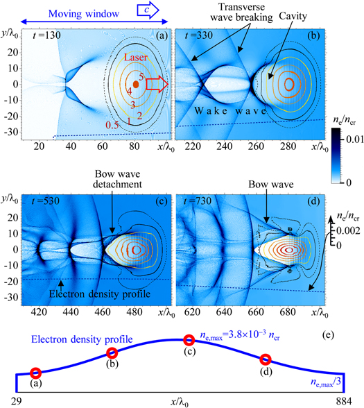
Figure 15. (a)–(d) 2D PIC simulation of laser pulse propagation in underdense plasma. The colour scale shows the electron density, the curves denote the isolines of the laser pulse dimensionless amplitude, and the blue dashed curve at the bottom of each frame shows the initial electron density profile. Spatial and temporal units are the laser wavelength and cycle period, respectively. The corresponding animation can be found in supplemental movie S1 (available at stacks.iop.org/NJP/16/093003/mmedia). (e) The initial electron density profile; the circles correspond to the laser pulse positions in frames (a)–(d).
Download figure:
Standard image High-resolution imageThe typical electron density distribution at the stage of the detached bow wave is shown in figure 16. This distribution is obtained in a 3D PIC simulation of a laser pulse linearly polarized along the y-axis, with a0 = 6.6, duration of 10λ0/c, and FWHM waist of 10λ0, interacting with a plasma of electron density ne = 0.001 ncr. The simulation is performed within the 125λ0 × 124λ0 × 124λ0 box with periodical transverse and absorbing longitudinal boundaries, with a resolution of λ0/32 along the x (propagation) axis and λ0/8 along the y- and z-axes. The number of quasiparticles is 2.3 × 10¹⁰. The laser pulse modifies the originally uniform electron density, creating the density modulations at the head of the pulse, the electron-free cavity with dense and sharp wall, and the bow wave. The highest electron density is at the joining of the cavity wall and the bow wave front, denoted as electron spike. Figure 16(a) also shows the region of intense high order harmonics generation with ω > 4ω0. This region coincides with the joining of the cavity wall and the bow wave, i.e. with the electron density spike. The generation of frequencies greater than ω0 can also be seen at the cavity wall and wake wave breaking and injection point; however, in the simulations presented here, at the highest frequencies corresponding to the experimentally observed high-order harmonics, the radiation from the electron spike is much stronger.

Figure 16. 3D PIC simulation results. (a) 3D distribution of electron density ne with the upper half removed; the density is shown with ray-tracing, the black contours correspond to ne = 0.0025ncr. The red arcs show the energy density of electromagnetic radiation with ω > 4ω0, i.e. the location of the high-order harmonics source. As the frequency increases, the length of the emitting arcs decreases. (b) The electron density distribution ne(x, y, z = 0) in the plane z = 0.
Download figure:
Standard image High-resolution imageIn order to simulate the emission of very high harmonic orders comparable to those obtained in the experiment, we performed a high-resolution 2D PIC simulation, figures 17– 20. The simulation was performed in a 87λ0 × 72λ0 window with a grid size of λ0/1024 along the x-axis and λ0/112 along the y-axis, with 6 × 10⁸ quasiparticles. The parameters of the laser pulse in the simulation are close to the parameters of the self-focused Astra Gemini laser pulse, i.e. a0 = 10, τ = 16λ0/c ≈ 43 fs, and a spot diameter of 10λ0 = 8 μm. The density of the plasma is ne = 0.01ncr = 1.7 × 1019 cm−3. The electron density profile shown in figure 17(a) contains all of the features described above, i.e. the cavity, cavity walls, bow wave, and the electron density spike. The density lineout across the spike is shown in figure 17(b); this data is taken ten cycles earlier than in (a) in order to demonstrate the structure of the spike responsible for the emission of the high-frequency radiation within the spectral range from 60ω0 to 100ω0 shown in (a) by the red colour scale.

Figure 17. 2D PIC simulation results. (a) The electron density ne (blue colour scale), isolines of the laser pulse envelope for the dimensionless amplitudes a = 1, 4, 7, 10, and electromagnetic energy density WH for frequencies from 60ω0 to 100ω0 (red colour scale). (b) The electron density profile lineout across the electron spike ten laser cycles earlier than shown in (a). (c) Profile of the right spike in (b) in the log−log scale, Δy = y − yC, yC ≈ 5 λ0.
Download figure:
Standard image High-resolution image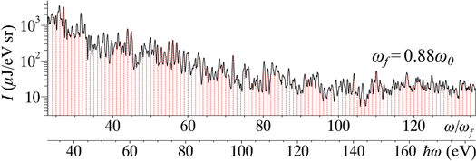
Figure 18. Emission spectrum of the upper spike in figure 17(a), black dotted rectangle.
Download figure:
Standard image High-resolution image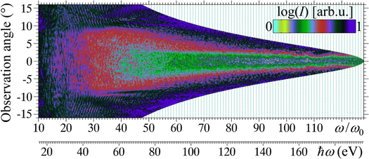
Figure 19. Angular distribution of spectral intensity in the grey dashed box in figure 17(a). The white area is beyond the simulation resolution.
Download figure:
Standard image High-resolution image
Figure 20. Multi-stream motion of the electron fluid corresponding to the simulation shown in figure 17. Each colour point represents one out of ten quasiparticles with the coordinates (x, y, y – y0), where y – y0 is the quasiparticle displacement along the y-axis from the initial coordinate y0. The colour encodes the initial distance |y0| of quasiparticles from the axis of the laser pulse propagation, as shown in frame (a) in the unperturbed region (x/λ0 > 15). The frames (a)–(d) represent different projections of the phase space. The animation showing the rotating phase space can be found in the supplemental materials of [26].
Download figure:
Standard image High-resolution imageThe profile of the electron density spike in the log–log scale is shown in figure 17(c). It is remarkable that the density growths as ∝(y – yC)−2/3 when the transverse coordinate approaches the spike location, yC. This power-law density dependence on the coordinate at the joining of two density walls, caused by a multi-stream plasma flow, is very characteristic, and gives an important clue to the mechanism of the electron density spike formation, see section 7.
The spectrum of harmonics in the region denoted by the dotted rectangle in figure 17(a) is shown in figure 18. The spectrum extends up to the ∼128th order, as is allowed by the simulation resolution. The emission is slightly off-axis, figure 19, with an emission cone size of several degrees. The spectrum of lower-order harmonics at the observation angle of 8°, obtained in the same simulation, is shown in figure 14(c). The off-axis angle decreases when the harmonic order increases. The harmonic energy yield obtained in the simulation is close to the experimental data obtained with the Astra Gemini laser, figure 12.
6. High-order harmonic generation mechanism
The electron density spikes at the joining of the cavity wall and bow wave move together with the laser pulse, and oscillate with the laser carrier frequency. With a linearly polarized pulse, the electron density spike is located at the crescent curves embracing the pulse head, figure 16, following the pulse electric field mirror symmetry. Circularly polarized pulses produce annular electron density spikes. At any time, the spike consists of different electrons, flowing in different directions through a curve embracing the laser pulse head, with momenta induced by the laser pulse field. As a strongly localized charge, oscillating with relativistic velocity, the spike emits electromagnetic radiation in accordance with classical electrodynamics [73, 77], in the form of harmonics with the base frequency equal to the local carrier frequency of the laser pulse. Owing to a strong spike localization, the short-wavelength radiation undergoes a constructive interference for electrons located at distances below a half-wavelength from each other. This radiation is coherent, and its intensity scales as a square of the number of emitting particles. We note that for constructive interference in the forward direction, it is sufficient that only the longitudinal size of the source is small enough in comparison with the emitted wavelength. In the simulations presented above, the number of electrons within the interval of width λ0/100 near the spike is Ne ∼ 106–107. With the emission intensity growing as Ne2, the spikes provide a signal level close to the experiment. The divergence of radiation is determined by the source size δ in the direction perpendicular to the observation direction, and by the source velocity with respect to the observer. The cusps move with relativistic velocity, which decreases the divergence angle by the Lorentz factor γ, i.e. Δθ ∼ λ/γδ.
In the region of the spike, the electron density is at a maximum in the direction of the electric field vector, since a greater amount of electrons are expelled in this direction. In the case of linear polarization, the maxima appear at a pair of opposite points, oscillating along the polarization axis. In the case of circular polarization, the maximum is located on a point travelling on a helical trajectory, following the electric field vector of the laser pulse. The coherent emission intensity strongly depends (as Ne2) on the number of electrons, therefore the higher the harmonic order, the smaller the emitting region near the electron density maximum.
The described mechanism is consistent with all of the features of the experimentally observed high-order harmonics. The strong localization of the electron density spikes removes the discrepancy between the estimated number of electrons which are encountered by the laser pulse, and the number of electrons emitted in a single-particle scattering regime required for the experimentally observed harmonic spectra. The electron density spikes are off-axis and therefore produce harmonics with both even and odd orders having the same shape and intensity.
The new harmonics generation mechanism is dominant when the laser pulse creates a bow wave while the accelerated electrons cannot produce coherent radiation. This is realized (1) in underdense plasma, ne < ncr, when (2) the laser dimensionless amplitude is much greater than 1, a0 ≫⃒ 1; (3) the laser pulse length is comparable with the Langmuir wavelength (so that the wake wave undergoes a transverse break in the first period suppressing electron self-injection into the wake wave); (4) the laser is tightly focused, making a spot with the diameter of  [36]. Under our experimental conditions, the large amplitude and tight focusing are achieved owing to relativistic self-focusing. These conditions remove or supress previously known harmonics generation mechanisms: atomic harmonics do not occur in plasma; accelerated electrons have too small a density and too large an energy spread so betatron emission is not coherent; all the electrons encountered by the tightly focusing laser pulse are transversely expelled, forming the bow wave and flow through the cusps (density spikes), so that their coherent cusp emission is always stronger than the nonlinear Thomson scattering.
7. Catastrophe theory model of the electron density spike formation
The formation of a strongly localized electron density spike and its peculiar properties, namely robustness to oscillations imposed by the laser field and the −2/3 power-law density dependence, can be explained with the help of catastrophe theory [27, 28].
The laser pulse expels electrons in both the longitudinal and transverse directions, while the electrostatic potential of the non-compensated background of slowly responding ions pulls the electrons back. This leads to a multi-stream motion of the electron fluid [76, 78], as is seen in figure 20, corresponding to the simulation shown in figure 17. As is shown in figure 20, the quasiparticles in the phase space (x, y, y – y0) are well-ordered according to their initial position y0 and are situated on a surface. Here  is the displacement along the y-axis from the initial coordinate y0, and γe is the electron Lorentz factor. The electron density increases abruptly at the location of the cavity walls and bow wave boundaries, representing catastrophes of the plasma flow.
The formation of catastrophes is illustrated by the following one-dimensional model of electron motion along the transverse coordinate y, figure 21 and supplemental movie S2 (available at stacks.iop.org/NJP/16/093003/mmedia). Initially, the electrons with spatially varied momentum  homogeneously fill the y-axis, figure 21(a). In the phase space
  , the phase 'volume' occupied by the electrons is represented in an implicit form by a curve
  . Due to the momentum inhomogeneity, the order of electrons eventually changes, thus a multi-stream flow arises and the curve S becomes folded. The electron density is obtained by a projection of the electron phase space onto the y-axis,

where ![$f\left( t,y,{{p}_{\bot }} \right)\propto \delta \left[ S\left( t,y,{{p}_{\bot }} \right) \right]$](https://content.cld.iop.org/journals/1367-2630/16/9/093003/revision1/njp499357ieqn9.gif) is the particle density in the phase space
is the particle density in the phase space  and δ is the Dirac delta-function. At the position of a fold, the density rises sharply. The emergence of a singularity in a flow is called a catastrophe. Note that in the case of the fluid approximation, projection (4) gives an infinite density, while in the case of a finite particle number, as in the supplemental movie S2 (available at stacks.iop.org/NJP/16/093003/mmedia), the density, although exhibiting a sharp rise, remains finite.

Figure 21. The model of electron flow with spatially varying momentum,  . The electrons occupy a phase volume represented by red thick curves in (a), (b) and (c) at different moments of time t. The projection of the phase space
  onto the y-axis produces the electron density ne(y), equation (4). The evolution of the initially homogeneous (a) distribution of electrons exhibits a consecutive formation of singularities in the electron density. The first singularity is neC ∝ (yC – y)−2/3 at the point y = yC (b), later it splits into two singularities of neF ∝ (yF – y)−1/2 at y = yF1 and y = yF2 (c). In the 3D phase space
  , the phase volume occupied by the electrons is surface S, frame (d). The formation of singularities in the electron density is seen here as the projection of the folds of the smooth surface S onto the (t, y) plane. The folds create the so-called fold catastrophe, while their joining corresponds to a higher order catastrophe, the cusp [27, 28]. The finite densities shown here correspond to a finite particle number, while the continuous fluid model gives infinite density values at the locations of the folds and cusp. See also supplemental movie S2 (available at stacks.iop.org/NJP/16/093003/mmedia).
Download figure:
Standard image High-resolution imageThe singularity type is determined by the structure of the phase 'volume'. By analogy with the observation that any smooth function at a regular point can be approximated by a linear form, in the general case, without special conditions on the shape of the curve S, a fold can be approximated by a portion of a parabola,

figure 21(c), while the portion near the curve S inflection can be approximated by a cubic,

figure 21(b). Therefore, the projection (4) gives the density singularity of

at the fold, and of

at the inflection point. In a higher dimensionality space  , the inflection point corresponds to a merger of two folds of a surface given by
  , figure 21(d). In the vicinity of the merger point,
  , the surface S can be represented implicitly by

with some constants α ≠ 0 and β ≠ 0 ([28], chapter 5 paragraph 2), in analogy with the approximations by a parabola and a cubic used above. Here the projection onto the (t, y) plane produces two singular lines joining at a point with a singularity of higher order. If we apply small smooth perturbations to the electron phase 'volume' represented by the curve S, the fold and the inflection still remain, and can be approximated locally by a parabola and a cubic, respectively. In other words, the corresponding singularities are robust with respect to the perturbations. The rigorous proof of this fact is given in catastrophe theory ([27], chapter 2; [28], chapter 6, paragraphs 4 and 5), which is a well-established branch of mathematics studying the formation of singularities in dynamical systems and in mappings. Here catastrophe theory establishes two structurally stable singularities, the fold catastrophe (A2, according to V I Arnold's classification) and the cusp catastrophe (A3).
Catastrophes of the same types as in the model in figure 21 appear in the laser plasma during cavity and bow wave formation [36], figure 22. Here the x coordinate of the laser pulse propagation corresponds to the reversed time in figure 21. The cusp catastrophe, appearing at the joining of the cavity walls and bow wave boundaries, figure 22(a), causes the formation of the electron density spike, figure 22(b), seen in the 3D PIC simulations, figure 16(b). The spike is located in a ring surrounding the cavity head, moving together with the laser pulse. Being pushed by the electromagnetic field of the laser pulse, the electrons form a flow modulated with the local laser frequency. Correspondingly, the electron spike undergoes periodic oscillations and emits electromagnetic radiation with high-order harmonics of the local laser frequency. Catastrophe theory ensures that the described singularities are structurally stable which means that they are insensitive to perturbations imposed by the laser pulse and other factors such as electron density fluctuations. Singularities stronger than the cusp can momentarily appear [78], however, they are not stable against the perturbations. Other singularities in collisionless plasma are discussed in [76, 78].

Figure 22. The catastrophe theory model. (a) The electron phase space (x, y, <py >), where <py > is the transverse momentum averaged over the laser period. (b) The electron density distribution ne(x, y) with singularities corresponding to the folds of the phase space, compares with figure 16(b). The electron density spikes appear at the places where two folds join, where the higher-order cusp singularities are formed.
Download figure:
Standard image High-resolution image
8. Harmonics generation scaling
Although the electron spike consists of different electrons constantly flowing through it, here we use a simplified model where the spike is considered as a point charge. The point charge approximation becomes better for higher order harmonics. According to classical electrodynamics [73], an oscillating charge emits harmonics up to the critical frequency ωc, corresponding to the critical order nHc, proportional to the cube of the particle energy εe. Assuming mostly transverse motion of electrons, where εe ≈ a0mec2, we obtain

At harmonic orders substantially higher than this, the spectrum exponentially vanishes, as observed in experiments. Assuming the stationary self-focusing condition, equation (2), we obtain the following scaling of the critical harmonic order, expressed via the laser peak power P0 and electron density ne:

where Pc is given by equation (1). We see that a 100 TW laser pulse with a wavelength of 1 μm, propagating in plasma with the density of 5 × 1019 cm−3 can produce at least about 250 harmonic orders.
The total energy εS emitted by the spike can be obtained using formulae from section 14.2 of [73]. It is proportional to the forth power of the charge energy, (a0mec2)4, and the charge squared, i.e. e2Ne2, and the emission time τH:

Here the harmonic base frequency ωf ≈ ω0. We take into account the relativistic motion of the charge, together with the laser pulse, and introducing factor γ, the Lorentz factor associated with the spike velocity, which is close to the laser pulse group velocity in plasma. The latter can be estimated in the first approximation as γ ≈ (ncr/ne)1/2. The stationary self-focusing condition, equation (2), and the relation between the emitting charge Lorentz factor and plasma density allows one to reveal the harmonic emission energy scaling. Equation (12) for P0 = 120 TW, ne = 1.9 × 1019 cm−3, Ne = 107 gives the total emitted energy of ∼1 mJ. Here we estimate a0 = aSF = 12, γ = 10, τH = 0.1 fs, using equation (2) and PIC simulation results. This energy corresponds to ∼60 μJ sr−1 in one harmonic (assuming that the divergence angle is ∼1/γ and the energy per harmonic is about total energy/a03), which compares well to the experimental value of 40 μJ sr−1 at 120 eV and the simulation result of 30 μJ sr−1 at harmonic order 100. For P0 = 9 TW, ne = 2.7 × 1019 cm−3, Ne = 106 the total emitted energy is ∼3 μJ. Here a0 = aSF = 6, γ = 8, τH = 0.7 fs. This energy corresponds to ∼1 μJ sr−1, in agreement with the experimental observation (∼1 μJ sr−1 at 80 eV).
9. Conclusion
We have experimentally discovered a new regime of high-order harmonic generation using multi-terawatt femtosecond lasers irradiating gas jet targets. The harmonics are generated by linearly as well as circularly polarized laser pulses in wide ranges of laser power and plasma density. The comb-like harmonic spectra containing even and odd orders extend to the 'water window' spectral region. The harmonics are emitted slightly off-axis with the emission angle reducing at higher orders. The harmonic yield grows faster than linearly with the laser power. We have proposed the harmonic generation mechanism based on self-focusing, following the nonlinear wake and bow waves excitation which produce electron density spikes coherently emitting high-order harmonics. Catastrophe theory explains the electron spike sharpness and stability. The maximum harmonic order scaling with the laser intensity will allow the attainment of the keV range. Our results open the way to a compact coherent x-ray or XUV source built on a university laboratory scale repetitive laser and an accessible, replenishable, and debris-free gas jet target. This will impact many areas requiring a bright compact x-ray or XUV source for pumping, probing, imaging, or attosecond science.
Acknowledgments
We acknowledge the financial support from MEXT, Japan (Kakenhi 20244065, 21604008, 21740302, 23740413, 25287103, 25390135 and 26707031), the JAEA Research and Development Adjustment Funding for Exploratory Research, the STFC facility access fund (UK), RFBR-JSPS collaboration program, Russia and Japan (RFBR Grant 14-02-92107) and Program for Basic Research No. 2 of the Presidium of the RAS, Russia.