


Abstract
Much effort has gone into identifying and classifying systems that might be capable of dynamo action, i.e. capable of generating and sustaining magnetic field indefinitely against dissipative effects in a conducting fluid. However, it is difficult, if not almost technically impossible, to derive a method of determining in both an absolutely conclusive and a pragmatic manner whether a system is a dynamo or not in the nonlinear regime. This problem has generally been examined only for closed systems, despite the fact that most realistic situations of interest are not strictly closed. Here we examine the even more complex problem of whether a known nondynamo closed system can be distinguished pragmatically from a true dynamo when a small input of magnetic field to the system is allowed. We call such systems 'stoked nondynamos' owing to the 'stoking' or augmentation of the magnetic field in the system. It may seem obvious that magnetic energy can be sustained in such systems since there is an external source, but crucial questions remain regarding what level is maintained and whether such nondynamo systems can be distinguished from a true dynamo. In this paper, we perform 3D nonlinear numerical simulations with time-dependent ABC forcing possessing known dynamo properties. We find that magnetic field can indeed be maintained at a significant stationary level when stoking a system that is a nondynamo when not stoked. The maintained state results generally from an eventual rough balance of the rates of input and decay of magnetic field. We find that the relevance of this state is dictated by a parameter κ representing the correlation of the resultant field with the stoking forcing function. The interesting regime is where κ is small but non-zero, as this represents a middle ground between a state where the stoking has no effect on the pre-existing nondynamo properties and a state where the effect of stoking is easily detectable. We find that in this regime, (a) the saturated state is somewhat unexpectedly enhanced by a bias resulting from the random fluctuating statistics of the decay process, and (b) the state is indistinguishable from a true dynamo except via κ itself. Such results make the pragmatic identification of dynamos in real situations even more difficult than had previously been thought.
Export citation and abstract BibTeX RIS

Content from this work may be used under the terms of the Creative Commons Attribution 3.0 licence. Any further distribution of this work must maintain attribution to the author(s) and the title of the work, journal citation and DOI.
1. Introduction
Dynamo theory is ubiquitously invoked to explain the presence of long-lived magnetic fields in many, if not most, astrophysical and geophysical situations, from the Earthʼs magnetic field through stars including our Sun and on to galaxies and other cosmological bodies. The support of a magnetic field against dissipative effects by the motion of an electrically conducting fluid is generally what is called dynamo action, and a magnetohydrodynamic (MHD) system that achieves a stationary magnetized state is called a dynamo. Since so much physics depends on this state, the search for general classes of dynamos has been quite intense. However, the identification and classification of dynamo systems is a difficult problem, particularly in the fully nonlinear regime.
Perhaps the largest body of work on classification and identification of dynamos relates to kinematic dynamo theory (see e.g. Stretch Twist Fold [1]). Here, the growth of magnetic field  from an infinitesimal perturbation is examined; the quadratic Lorentz force is negligible, and consequently the momentum and induction equations are decoupled. One can therefore choose any flow and solve for the magnetic field. The induction equation is linear in
  , and the presence of an exponentially growing mode clearly identifies the system as a kinematic dynamo. Of course, the growth of the field quickly leads to amplitudes that render the kinematic approximation invalid. It is typically assumed that then the Lorentz force saturates growth, but the transition to nonlinearity and the subsequent long-term maintenance of field can be studied only by solving the fully coupled momentum and induction equations.
In attempting to classify dynamo systems in the nonlinear regime, some intrinsic difficulties are encountered. No longer can the velocity simply be specified. It is prudent instead to specify the forcing that is applied to the momentum equation, for that can persist unchanged throughout the evolution. One approach is to tailor it to make the desired target flow a solution of the momentum equation in the kinematic regime. An advantage of so doing is that the nonlinear calculation can then be compared with a well studied kinematic system. However, complications arise because the target flow may be neither a unique nor a stable solution to the forced problem, and the flow actually realized in the nonlinear regime may be quite different from the desired target.
Other issues further cloud the nonlinear problem. For example, no system can be observed indefinitely. Magnetic decay times can be too long for practical observation, rendering the matter unresolvable (indeed, the molecular magnetic diffusive timescale for a star may be greater than the starʼs lifetime on the main sequence [2]; even turbulent decay, which is expected to be much faster, may be slower than what one might anticipate from a naive analysis of the hydrodynamic turbulence, since the magnetic field is not passive, and modifies the flow [3]).
Here, we consider an additional complication. The MHD systems adopted for dynamo calculations are typically magnetically closed, having no imposed source of magnetic energy apart from the initial field. This is true of both analytical and numerical work, in which idealized boundary conditions are conveniently imposed. Realistic situations, however, are generally subdomains of much larger systems, and are typically not completely isolated. Transport of magnetic field into the region is thereby permitted. Thus we ask: Is it then possible for a region that in isolation is not a dynamo system to be maintained in a state indistinguishable from a true dynamo when it is supplied from outside with a magnetic field? Answering that question is a challenge that has been issued in the context of solar dynamo theory [4], where primordial magnetic field deep in the radiative zone may leak into the tachocline, a region of potentially strong magnetic field amplification. That challenge is taken up here.
It may seem obvious that an external source can support magnetic energy in a system, but the real question of interest concerns more the level at which magnetic energy can be maintained, and whether the external source is detectable from measurements within the region. Consequently, we study systems that are intrinsically nondynamos in isolation, and examine whether a weak magnetic source can support the system in a nonlinear state that mimics a true dynamo. We call our supported systems 'stoked nondynamos'. If in practice such false dynamos cannot be separated from true dynamos without independent knowledge of the existence of an external source, new and potentially interesting avenues of exploration may be opened.
In this first paper, we work with systems, previously studied in detail by Brummell, Cattaneo and Tobias (BCT) [5], which are well known for their kinematic dynamo properties and which are easily integrated into the nonlinear regime. This paper therefore serves as a highly idealized proof-of-concept. In a subsequent paper, we examine more realistic scenarios and 'essentially nonlinear' dynamos, in which the Lorentz force acts not only to saturate any linear growth but actually drives flow that contributes to dynamo action. Although the issues outlined above apply to all dynamos, in this paper we work specifically with examples of small-scale dynamos, where the magnetic field is created at scales comparable to those of the velocity field (and smaller) rather than with large-scale dynamos that generate fields at scales significantly larger those of the velocity.
2. Formulation
The investigation reported in this paper concerns forced, incompressible MHD in the triply-periodic Cartesian domain  . The governing equations are:


Here  is velocity and
  is the magnetic field; both are measured in the same units. The equations have been nondimensionalized with a typical velocity U and length scale L, and depend on the dimensionless Reynolds number
  and magnetic Reynolds number
  , where ν and η are the (constant) kinematic viscosity and magnetic diffusivity respectively. Throughout this paper, as in BCT,
  .
.
The terms  and
and  represent the forcing:
  is the main driving force,
  the rate of magnetic leakage into the system; clearly both terms inject energy. Here, following BCT, we set

in which  with
with
The target flow  adopted here (and in BCT) is a time-dependent version of an ABC flow, with
  , where Ω is the frequency and
  the amplitude of a harmonic displacement of the origin of the ABC flow along the line
  . This flow is maximally helical, so it can easily be shown that
 ![$\nabla \cdot \left[ ({{{\vec{u}}}_{{\rm T}}}\cdot \nabla ){{{\vec{u}}}_{{\rm T}}} \right]\equiv \vec{0}$](https://content.cld.iop.org/journals/1367-2630/16/8/083002/revision1/njp498551ieqn17.gif) , and therefore, in the absence of magnetic field and hydrodynamic instability,
, and therefore, in the absence of magnetic field and hydrodynamic instability,  would drive the velocity field toward the prescribed target flow. This forcing is chosen over, say, stochastic forcing, owing to its known and easily controllable nonlinear small-scale dynamo properties, as outlined in the next section.
The magnetic forcing term  is constructed similarly: it takes the form

and we choose  with
with
Here, B0 is the amplitude and k is the wavenumber of the stoking magnetic field that is leaked into the domain. In the absence of fluid flow,  would drive the system from arbitrary initial conditions toward the steady target magnetic state
  on a diffusive timescale. However, we emphasize that, in general, significant flow fields are likely to be present, and the specific magnetic configuration suggested by equation (7) would never actually be realized. The important property of the stoking term is then that it provides a way to augment the magnetic field incrementally in the system. This is done volumetrically rather than through the boundaries, owing to the periodic nature of the problem. This method of forcing is capable of acting in an anti-diffusive or positively diffusive manner depending on the alignment between the augmented field and the original field, as we shall see later. Notice that the forcing adds no net flux to the system, that the injection length scale is directly controllable but is of the box (and velocity) scale or smaller, and that the augmented field is non-helical. Forcing in the induction equation has been used previously in problems where the generation of magnetic field at scales much larger than the velocity scale is of interest (the 'large-scale dynamo' problem) and there the helical nature of the forcing is important (see e.g. [6, 7]). In the small-scale dynamo problem examined here, this is not of importance. Furthermore, we anticipate being most interested in cases where the injected magnetic energy is small compared to the kinetic energy of the forced flow, and so flows driven by the injected field are relatively unimportant for induction, although this must be checked a posteriori.
The numerical code used to solve the equations employs a standard  -dealiased pseudospectral method [8]. The solenoidal conditions on both the velocity and magnetic fields (equations (1)) are enforced by using a poloidal and toroidal decomposition of both the velocity and magnetic fields and solving for the evolution of these scalar potentials. Time updates are performed using an explicit 3rd-order-accurate Adams–Bashforth scheme. All simulations reported here were run on a 963 grid.
3. Nondynamo solutions to the unstoked problem
We summarize the pertinent aspects of the nonlinear (unstoked:  ) solutions found by BCT, which serve as initial conditions for our stoked calculations: if and Ω are set to zero, the target velocity reduces to a standard ABC flow with
  , a flow that is known to be mostly integrable with small regions of chaoticity. The dynamo properties of this system have been studied quite extensively [9–16]. If both and Ω are nonzero, the target velocity is essentially the same flow oscillating along the line
  . The regions with chaotic streamlines are now considerably enlarged, providing much better conditions for dynamo action. Information about the detailed behaviour of this system and its sensitivity to and Ω, including kinematic dynamo properties and the subsequent nonlinear evolution, can be found in the BCT paper [5]. In the remainder of this paper, we confine ourselves to
  , and we use Ω as our control.
BCT showed that the nonlinear behaviour of the system depends strongly on Ω. Results from two simulations of particular interest, exhibited by BCT and recalculated here with a different numerical code, are shown in figure 1(a). The plots show the time series of a good tracer of dynamo activity, the spatially-averaged magnetic energy density, E (where  with V the volume of the computational domain; denoted as
  later in the paper). When
  , the long-term nonlinear MHD state is statistically stationary, and is a fine example of a small-scale dynamo; when
  , however, despite an initial kinematic amplification similar to that when
  , the subsequent nonlinear state is not maintained, but instead decays.

Figure 1. Plots of spatially-averaged magnetic energy density E for three different unstoked cases. Both plots show the Ω = 1.0 dynamo for reference, with the system saturating at a significant fraction of equipartition. (a) Shows the continuous decay of the Ω = 2.5 case at a rate close to the expected Ohmic value. The straight dot-dashed line on both plots exhibits the Ohmic dissipation of a fundamental eigenmode in the absence of fluid motions. (b) Shows the much slower overall decay of the  case, incorporating randomly alternating periods of growth and decay. As in all simulations,
  and the box has dimensions
Download figure:
Standard image High-resolution imageBCT explain that there is a magnetically driven transition from the hydrodynamic state ( in BCT; our
  ) producing the exponential amplification to an MHD state with a different velocity field (which BCT called
  ). The final hydrodynamic state is not a kinematic dynamo when
  , but it is when
  . Details of the cause of this behaviour are not important for our discussion here, and we simply emphasize two points. The first is that this property provides us with a convenient medium for generating self-consistently two nonlinear MHD states, of which one supports magnetic field (i.e. is a nonlinear dynamo) and the other does not (i.e. is a nonlinear nondynamo). That justifies our ignoring the details of the amplification phase, which we simply regard as a means of obtaining our initial MHD conditions. The second point is that, as discussed by BCT, the new underlying hydrodynamic state
  is hydrodynamically stable, and does not revert to the original state
  when the magnetic field decays to negligible values: our chosen
  is magnetohydrodynamically unstable, and the flow to which it evolves is not a dynamo. The transition is permitted because we specify a forcing and not the flow field. Thus we see that
  is an interesting parameter range for more detailed study.
In surveying that range, we found that the highest modulation frequency displaying clear dynamo activity is  ;
;  was the lowest frequency with a clear decay. Figure 1(b) illustrates an intermediate system, at
  . It appears to be marginal , in the sense that it is uncertain within the time span of the simulation whether the magnetic field would ultimately decay or be sustained; it is evidently not a simple stationary saturated dynamo as in the case
  , since the system fluctuates far more wildly yet does not conclusively decay. The time series of the magnetic energy density E has a broad spectrum of growing and decaying fluctuations, typified by very rapid bursts and longer periods of Ohmic-like decay (where the Ohmic diffusion timescale
  here).
The  system illustrates well the complexities to be faced when trying to decide whether a system is truly a dynamo or not. Since marginal situations such as this present significant difficulties for assessment, we shall not concentrate on them here, but instead devote most of our attention to the stoking of clear nondynamos, and to comparing their behaviour with that of clear dynamos.
4. Stoking nondynamos
We choose the system with  as our canonical example of a nondynamo. In this system we include
  in equation (3) with a non-zero B0. We then attempt to address three fundamental and related questions.
- (i)Can stoking counteract natural decay well enough to sustain magnetic activity?
- (ii)Is any observed level of saturation significant and interesting?
- (iii)Can stoked nondynamos be distinguished by any practical means from true dynamos?
4.1. Results
The answer to the first question is obviously, and almost trivially, affirmative. Although the stoking considered here imparts no net flux to the system, it does add magnetic energy, making continuous decay impossible. To demonstrate this, we examine four stoked cases at  , in which the stoking amplitude B0 is varied through the values
  ; the wavenumber of the magnetic forcing k is set to unity. The system is started from rest with an initial weak seed field of random orientation, and random amplitude with zero mean and maximum value 10−5 at each grid point. The velocity field starts from rest, and each simulation uses identical initial conditions, the only difference between them being the stoking amplitude B0.
Figure 2 shows for the four cases the evolution of the mean magnetic energy density E, a typical measure for detecting the presence of dynamo action. Each simulation goes though an initial amplification phase that is nearly identical to that in the unstoked case (except that, at very early times, additional linear growth resulting from the stoking can be discerned on closer examination of the data in figure 2). Again, we stress that these initial phenomena are not of real interest in the current problem; indeed, it may even have been more perspicacious merely to have switched on stoking in the established nonlinear regime of the BCT cases. After the amplification process has saturated the magnetic field starts to decay away, as before in the corresponding unstoked case. The effect of the stoking comes into significance only in the longer-term evolution. Whereas continual decay would ensue in the unstoked system (figure 1(a)), all the stoked cases instead equilibrate to some statistically stationary MHD state with a mean magnetic energy density that depends upon the stoking amplitude B0. The time taken to reach that state also depends on B0. We have estimated by the vertical dashed lines in figure 2 (somewhat arbitrarily, but taking heed of any large temporal variations in E that may be present) the time at which stationary states may be considered to have first appeared. Any average over the stationary states reported in the rest of this paper begins at this time. The horizontal dotted lines denote a saturation amplitude that one might predict through a simple balance of the stoking term against turbulent decay; it will be discussed in detail in the next section. Whilst some simulations (e.g.  ) suffer more prolonged excursions of E, each comes to a saturation level that seems to scale more-or-less with
  . The saturation level is robust, being the same for any given B0, irrespective of the magnetic or hydrodynamic initial conditions adopted.
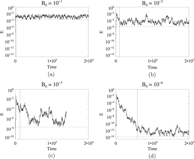
Figure 2. Time series of E for stoked cases with  and
and  . Vertical dashed lines show the delimitation between when the system is considered decaying and considered saturated. Horizontal lines show expected saturation levels when using a simple balance between the magnetic forcing and the unstoked decay rate.
Download figure:
Standard image High-resolution imageThe proportionality of the saturation level to the strength of the stoking is entirely expected. What remains to be determined is the constant of proportionality, and whether the stoking alters the system in a way that is readily detectable. We therefore need a baseline understanding of what might and might not be expected. That we now pursue.
4.2. Analysis
It is clear that there are at least two competing processes active in the simulations. The baseline system, driven by  but unstoked, is a nondynamo, whose transient field decays over long periods of time. The stoking,
  , adds field to what would otherwise become a magnetically free domain. The levels of magnetic energy density E at which these two processes balance can be used to judge whether any other interesting processes are occurring, and whether the saturation levels are significant. We stress again that
  imparts zero net flux, and is capable of removing field as well as adding to it, so some care is required in the treatment that follows.
We begin by extracting an intrinsic decay rate from the unstoked system. We integrate the unstoked system for an exceptionally long time, as indicated by figure 3(a). It immediately becomes clear that there is no single, well-defined, representative exponential decay rate, as is evinced by the various fits, depicted by the dashed lines, to different sections of the data. The instantaneous decay rate  changes rapidly, and even includes transient periods of growth, thus making any reference to λ as a 'decay rate' somewhat obscure. We shall define λ technically as a growth rate, with negative values indicating decay, although, as it is commonly negative over long periods of time, we often nonchalantly refer to it as a decay rate. Figure 3(a) suggests that the general rate of decay decreases as the magnetic field decays, however, this is merely a feature of this particular realisation of the chaotic system.

Figure 3. (a) Shows a very long time series of E for the unstoked  case. The dashed lines show fits to various sections of data, exhibiting the range of possibilities for an estimate of the decay rate. (b) Shows the spectrum of growth and decay rates calculated from the data in (a). (c) Shows the distribution of growth and decay rates found after filtering the forcing oscillations out of the data.
Download figure:
Standard image High-resolution imageIn figure 3(b) is displayed the total spectrum of growth and decay rates, calculated by taking the log of the data in figure 3(b), approximating the derivative with a simple first-order difference, and then taking the Fourier transform. There are three distinct peaks: the center peak corresponds to the frequency Ω of the forcing in the momentum equation, the right peak is the second harmonic, resulting from a quadratic quantity; the peak on the left contains all the variation of principal interest. Figure 3(c) depicts the distribution of the growth and decay rates obtained, after filtering the data with an upper cutoff at frequency 0.2 to eliminate unwanted signal from the forcing. The resulting data behave in a more-or-less Gaussian manner, having a mean growth rate  (i.e. a decay) and standard deviation
  . The latter is considerably larger than the mean, reflecting the large transient excursions, including significant growth periods, which make it difficult to discern the average behaviour.
We derive a formal definition for  in the unstoked case as follows. Using
  and
and  to denote spatial averages over the domain and temporal averages over the entire simulation respectively, we take the inner product of the induction equation with
  and average spatially to provide an evolution equation for the average magnetic energy density E:

Dividing by E gives the evolution equation for  , which is equivalent to an instantaneous growth rate
  :
:
Time averaging the resulting left-hand side is exactly equivalent to the  described above:
We proceed in like manner with the induction equation in the stoked system. The only resulting difference is that an additional term from the stoking appears, and, assuming that the system is in its saturated stationary state, the time derivative on the left-hand side of the new equation should time-average to zero; thus
Equations (10) and (11) share a term with a common mathematical form. However, since the two forced systems are fundamentally different, it is unclear whether there is a straightforward relation between them. To progress, we can make the simple hypothesis that the statistical properties of this term carry over from the unstoked to the stoked system. This essentially presumes  to result from a turbulent dissipation that is characteristic of the hydrodynamic specification of the problem. In particular, it implies that the magnetic field in the stoked problem is weak enough not to affect the underlying velocity fieldʼs characteristic turbulent dissipation. We shall formalize the conditions for the veracity of this hypothesis shortly.
We now substitute  from equation (10) into (11), resulting in an equation describing the stationary state of a stoked simulation:
Here, the numerator of the rightmost term represents an average alignment or correlation between  and the stoking term
  . We define a normalized version of the correlation coefficient as
where  is the rms of the magnetic stoking term. This quantity is key to our hypothesis, and essentially determines the regime of greatest interest, by representing the degree of influence of the stoking on the resultant field. If the stoking and the resultant field were completely uncorrelated, κ would average to zero, and the system could not exist in the stationary state described by equation (11); instead it would revert to the decaying dynamics dictated by equation (10). When
  there can be no equilibrium; on the other hand, large κ represents situations in which the resultant field is correlated significantly with the stoking, and therefore should be detectable. Evidently, in the regime of interest, κ is small but non-zero: the stoking has some influence on the system, and a stationary state can thereby be achieved, although the signature of the stoking is not so great as to be detectable. In this regime, our hypothesis regarding the transferability of the statistics between the two systems and the use of the unstoked
  in equation (12) should then be reasonably secure.
If we assume further that we can regard κ as being constant during the saturated phase of the stoked system, equation (12) can be written as

At first we limit ourselves to k = 1—we shall discuss the effect of varying k later—and rearrange this expression in terms of the expected level for the average magnetic energy density:
This quantity is to be compared with the equivalent measure derived directly from the actual system;

This definition of  may seem somewhat unwieldy, but it does provide us with a quantity that is consistent with equation (15).
If saturation really does result from a simple balance between  and the nondynamo nature of the unstoked system, these two quantities,
  and
and  , should be equivalent. It should be stressed that, while
  has an explicit dependence on
  , that dependence is due solely to the manner in which the stoking
  has been formulated. In the present system, magnetic field is being imparted on a diffusive timescale, but were any other timescale considered, it would appear in the formula for
  , and dependency on
  would be implicit.
We have tested our expectations by calculating  and
and  from our suite of simulations. Values of κ were evaluated explicitly according to equation (13) over the periods of saturation (i.e. from the dashed line in figure 2 onward), and then averaged over time. In table 1 are listed the time- averaged values
  so derived, together with the associated standard deviation
  of that measured mean.
Table 1.
Measured list of simulations. Reported here is the mean decay rate  of the unstoked system, the mean alignment
  and its measured variance
  , the measured saturation level
  and the predicted saturations
  which use the average and simulation specific κ values respectively. For all simulations,
  and the box has dimensions
| Run | B0 | Ω | k |

|

|

|

|

|

|
|---|---|---|---|---|---|---|---|---|---|
| 1 | 0 | 1.0 | 1 | 
|
−0.012 | 0.013 | — | — | — |
| 2 | 0 | 2.5 | 1 |

|
−0.004 | 0.01 | — | — | — |
| 3 | 0 | 2.0 | 1 |

|
−0.008 | 0.013 | — | — | — |
| 4 | 0 | 1.7 | 1 |

|
−0.001 | 0.004 | — | — | — |
| 5 | 10−1 | 2.5 | 1 |

|
0.086 | 0.0041 |

|

|

|
| 6 | 10−2 | 2.5 | 1 |

|
0.064 | 0.0040 |

|

|

|
| 7 | 10−3 | 2.5 | 1 |

|
0.034 | 0.0041 |

|

|

|
| 8 | 10−6 | 2.5 | 1 |

|
0.077 | 0.0042 |

|

|

|
| 9 | 10−3 | 2.5 | 5 |

|
0.198 | 0.124 |

|

|

|
| 10 | 10−3 | 2.5 | 10 |

|
0.571 | 0.139 |

|

|

|
| 11 | 10−3 | 2.5 | 15 |

|
0.582 | 0.263 |

|

|

|
| 12 | 10−1 | 2.0 | 1 |

|
0.081 | 0.0080 |

|

|

|
| 13 | 10−2 | 2.0 | 1 |

|
0.054 | 0.0094 |

|

|

|
| 14 | 10−3 | 2.0 | 1 |

|
0.053 | 0.010 |

|

|

|
We first verified the expected null correlation in the unstoked cases by dotting the observed magnetic field with the  that had been used in the stoked simulations. Table 1 shows that for these simulations (1–4) the deviation in the measured mean alignment is as large as the value itself, and thus the mean is consistent with zero. That cannot be true of the stoked systems, however, where continuous decay is not observed; indeed it can be seen that the values of
  in all the other simulations differ significantly from zero. There is no obvious identifiable systematic trend with the variation of B0, at least when k = 1 and
  . A variation of
  with k is apparent, however, and this will be discussed later. We note that the presence of large values of κ would invalidate our earlier analysis, and then we would not expect
  to equate to
  ; such entries are included in the table for completeness.
When using equation (15), we adopt an appropriate  for the underlying hydrodynamic system (e.g.
  for
for  as reported earlier), and we either adopt the values of the alignment
  calculated for each case, to give
  , or instead assume some universality of κ in the face of a lack of obvious trends, and use the average value over all the simulations calculated with k = 1, to give
  . The latter value turns out to be
  ; the individual values can be gleaned from the table.
Figure 4 is a graphical representation of the key data in table 1 for  . Most interestingly, there is always a factor 10 or more discrepancy between either of the saturation values (
 or
or  ) predicted by the simple arguments above and the actual measured saturation value (
 ), regardless of the stoking amplitude B0. This is not true only of this particular case: by examining entries in table 1, one can verify that the same is true for
  , for example. The excess over our simple expectations appears to be a robust feature of stoked nondynamos of this type. It implies one of two things: either our assumptions in calculating
  are wrong, or that other processes are present and the observed saturation levels are indeed significant. Using the data above and a simple model, we now demonstrate that the latter is true, and that under certain conditions a systematic bias towards elevated energy levels can arise.
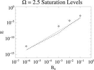
Figure 4. The dotted line represents the predicted saturation level  using relation (15) and using the average κ. The dashed line shows the predicted value
  using the case specific
  . The symbols mark the observed saturation levels
  from (16).
Download figure:
Standard image High-resolution image4.3. A systematic bias
Further information is acquired by varying the wavenumber k of the magnetic forcing function (7). Simulations 7 and 9–11 listed in table 1 were carried out at the same forcing frequency,  , and the same stoking amplitude,
  , but with
  . We see that the measured value of κ increases sharply with increasing k; it is the only readily discernible trend in the κ data.
Additionally, figure 5 depicts time series of E stoked at these four different wavenumbers. The horizontal line in each plot represents the predicted saturation level  calculated using the universal value
  distilled from the previous k = 1 results. Two further interesting observations can immediately be made from these plots. First, as the wavenumber of the forcing is increased, the saturated state becomes much less intermittent. Second, at higher wavenumber the average magnetic energy is closer to the predicted value
  . The latter observation appears to contradict our first observation that κ was large for large k, since we expect large κ to invalidate equation (15). This can possibly be reconciled by recognising that our observed
  has an implicit k2 dependence being representative of a diffusive process and therefore EP should plausibly always be independent of k. Regardless, what is most interesting is that these results clearly demonstrate that the saturation magnetic energy is elevated by transient processes, and that these processes are more effective when k is small.

Figure 5. Average magnetic energy densities for  and various values of k. The predicted saturation amplitude lies just below the bulk of the data for all simulations. For (c) and (d) the temporary spikes in amplitude cease and the time series comes to a more steady stationary state.
Download figure:
Standard image High-resolution imageThe occurrence (or not) of strong transient excursions can be explained in terms of the relative scales of the fluid and the stoked input field: in our analysis of the unstoked decay we emphasized that the system experiences periods of intermittent growth, during which the energy augmentation by field folding dominates over the consequent increased dissipation. A characteristic turbulent inverse length scale pertaining to this process can be estimated as the average over space and time of  . In the simulations it is found that
  . When the stoking scale is larger than the velocity scale (
 ), the magnetic field appears smooth on the scale of the motion. Then field amplification can occur during transient periods when the growth rate is positive. On the other hand, when
  , the magnetic field appears corrugated relative to the velocity scale, so typically the fluid is merely advecting field without significant distortion, and therefore diffusive loss is not compensated by enhanced field stretching, no matter what the flow topology.
The transient growth rates that this system exhibits are clearly an important feature. While the decay of the unstoked system can be described fairly accurately using the mean decay rate alone, it is not clear how the full statistics carry over to predictions of behaviour in the stoked case. We now see that, in the stoked systems, the variance inherent in the decay rate may allow an augmented saturation compared to what might be expected from a simple balance between the average dissipation rates in the system and the applied stoking. We here explicitly exhibit this issue by building a simple toy model that forces the assumptions of our estimations in equation (15) to be valid and examines purely the effect of transient growth.
We achieve this by constructing an artificial time-dependent  as follows, instead of using a simple mean λ. A random sample of values is selected with the same Gaussian distribution (same mean and variance) that was extracted from the decay of an unstoked simulation (e.g.
  ; see figure 3(b)). Each of these is retained for a fixed
  consistent with the filter width used to produce the distribution (e.g.
  for the distribution shown in figure 3(c)). Given
  , one can then compute a time series for the average magnetic energy density from

using existing values for the correlation  from a simulation. One realisation of this process is shown in figure 6 with a
  that mimics the statistics from the unstoked simulation with
  and using the correlation statistics
  from the stoked simulation at parameters
  . The value
  predicted by equation (15) is marked with a dotted line, and the actual measured
  is marked with a dashed line. Clearly,
  errs on the low side, and the true mean value
  of the time series is elevated by the bias imposed by of the extended growth periods. The discrepancy can be accounted for only by the effects of the transient growth inducing significant deviation from a simple balance between stoking and intrinsic decay; it cannot be a result of improper flow statistics. Replacing
  with the mean κ has no significant effect, thereby providing further supporting evidence for the dominant effect of the variance of
  .
.
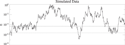
Figure 6. Simulated data generated by solving equation (17). The measured mean magnetic energy density is roughly an order of magnitude larger than what is predicted by equation (15).
Download figure:
Standard image High-resolution imageThis proof-of-concept toy model is not to be taken too literally. Its properties are quite sensitive to whether  is chosen self-consistently, and clearly
  should not change on regular time intervals, nor should its values in different intervals be independent. However, the exercise here forced the statistics of the decay rate in the stoked system to be exactly the same as in the stoked system, and an increased saturation was still observed. This can be understood intuitively by considering the implications of a varying
  . Because
  varies inversely with λ, the effect of two equal but opposite perturbations to the decay rate about its mean average out to favour an
  above
above  . Any transient positive growth rate
  could in principle cause unbounded growth (unless nonlinear effects cause saturation), whereas transient decay
  is bounded below by
  . The ultimate conclusion is that transient growth due to fluctuating flow properties has an important effect in the system.
5. Distinguishing stoked and dynamo states
We have established that the stoked simulations can sustain a significant magnetic field. The question remaining is whether these states can be distinguished from true dynamos. One might envisage having snapshots, or even movies, of the magnetic field on some exterior surface, or time traces of various scalar proxies for the magnetic energy. We have found that, even when considering detailed structural information which in practice no observer could possess, it would be difficult, perhaps impossible, to distinguish between a stoked nondynamo state and an unstoked true dynamo.
To facilitate the investigation, we introduce two new simulations with very strong stoking: we consider magnetic forcing amplitudes  , at k = 1 and with our canonical nondynamo forcing frequency
  . Figure 7 shows the evolution of the magnetic energy density in the new simulations; they are to be compared not only with the more weakly stoked simulations already discussed, but also with the reference dynamo solution at
  The new simulations are forced unreasonably strongly for representing any practical situation; they are included for comparison between stoked systems in which the field might be dynamically very important and the more nearly kinematic, weakly stoked, systems. The former fall into the large- κ regime, whereas our previous simulations were mainly in the small-κ regime. As is evident in figure 7, the
  simulation sustains a magnetic energy density comparable to the dynamo case; the
  case is even stronger. In these cases, since κ is not small, the flow statistics are disturbed by the stoking, which is why they were not included in our earlier discussion. Indeed,
  in these stronger systems overestimates the saturation magnetic energy density significantly, although the systems do still saturate.
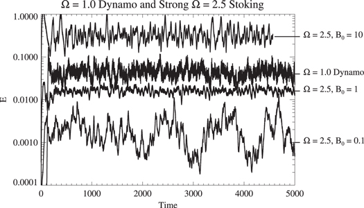
Figure 7. Time series of the magnetic energy density for strongly stoked  systems. Two cases are shown for stoking amplitudes
  and B0 = 10, demonstrating that the systems respectively saturate at magnetic energies close to and beyond that of the reference natural dynamo system at
  (shown as the dotted line; second from the top). Also included for reference is the
  stoked simulation from earlier (bottom line).
Download figure:
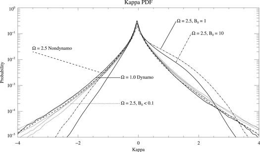
Standard image High-resolution imageSome of the stoked systems do equilibrate at relatively weak levels of magnetic energy, far below equipartition, but this can be a property of a true dynamo too (e.g. the  marginal dynamo of figure 1(b)). Furthermore, neither the fieldʼs spectrum, nor its other statistical properties, nor any general anisotropy, could distinguish between stoked nondynamos and true dynamos in their respective saturated states. Since these findings are negative, we refrain from elaborating on the evidence. The one detectable bias that we have seen, even at weak levels of stoking, is in the probability density function of a pointwise measure of κ, illustrated in figure 8. This κ is measured as in equation (13), save that no spatial averaging was performed. The PDF from the
  dynamo system seems to be symmetric, as would be expected of any unstoked system on which no biased external influence has been imposed. For all of the stoked cases, however, the PDF is suppressed at negative values of κ, and augmented at positive values. The bias in the weakly stoked simulations is small, as would be anticipated from the small values of
  listed in table 1.
Figure 8. Shown are PDFs of κ which were calculated using a pointwise version of equation (13). The solid line is the  dynamo and the dashed line is the
  nondynamo. The dotted lines are the weakly stoked cases with
  and the dash-dotted and dash-triple-dotted lines are the strongly stoked cases with
  respectively.
Download figure:
Standard image High-resolution image
That a bias can be detected through κ is almost tautological. By design, κ distinguishes between strongly (κ large) and weakly (κ small) influenced systems, and those without any stoking ( ). The small-κ regime is not only one where our earlier analyses apply, but is also where the stoking is virtually undetectable. High levels of stoking may be detectable in the numerical simulations via κ, but such systems are unlikely to arise in practice. Nonetheless, regardless of its behaviour, κ is not a practical observable in real situations. It seems that differentiation at plausible levels of stoking would be virtually impossible with the limited observables available to real astrophysical systems. For all intents and purposes, stoked equilibria look like dynamos.
6. Conclusions
We have studied the effect of adding 'external' magnetic field to a system which, when closed to external sources, has known nondynamo properties. The system is a forced triply-periodic electrically conducting fluid in which, in the absence of any magnetic field and instability, a time-dependent ABC flow is driven by body momentum forcing. The associated MHD system has known small-scale dynamo properties in the (linear and) nonlinear regime (see BCT). In particular, there is a range of oscillation forcing frequencies Ω in which the system is known to vary between a stationary dynamo state ( ), through a marginal dynamo (
 ) to a clear nondynamo MHD state which eventually decays to a virtually hydrodynamic state (
 ). To mimic the transport of external field into the closed system, or 'stoking' as we call it, an extra magnetic forcing term is added to the induction equation which creates a desired field volumetrically at a chosen rate. We examine the question of whether nondynamo systems, when 'stoked' with a small amount of extra field, can achieve stationary MHD states, and whether they are potentially distinguishable from true dynamo states.
In the case of an original unstoked system with clear nonlinear nondynamo behaviour (e.g.  or
or  ), stoking the system can indeed lead to a nonlinear stationary MHD state reminiscent of a dynamo. The existence of such a state might seem obvious, since one would expect the natural decay of the nondynamo system to be countered by the rate of input of the external field. We show that, if the statistics of the unstoked case can be carried over to the stoked system—a key assumption—the saturation state can be quantified via a correlation coefficient κ that measures the normalized projection of the resultant magnetic field onto the forcing. This effectively indicates the degree of influence of the forcing. The regime of interest is where κ is small, and the influence of the Lorentz force on the flow is not too great. In this regime the differences between the stoked nonlinear state and a true dynamo state are undetectable by any practical procedure. It appears that the only quantity that reveals the stoking is κ itself, and that is inaccessible in realistic systems in any pragmatic sense.
In the small-κ regime, the measured level of saturation  is generally at least an order of magnitude higher than the value of
  predicted by these simple ideas. We have shown that these elevated saturation levels are not a result of the unreliability of the assumptions made in the prediction, but rather the outcome of an interesting system bias related to strong fluctuations of the growth and decay rates inherent in the unstoked system. Even when deviations from the mean decay rate are equally distributed, intermittent transient (and unbounded) growth leads to greater production of strong field than removal, thereby elevating the saturation levels. We have demonstrated this process with a simple model. Not only are the stoked stationary states indistinguishable from true dynamo states, but also they can exist at surprisingly high levels of magnetic energy. This bias could be considered as another example of transient growth due to non-normality of the induction operator as expounded in, for example, [17], although those studies concentrate more on optimal excitation and noisy input rather than the weak, laminar energy source studied here.
The large-κ case, where the magnetic forcing affects significantly the statistics inherited from the background unstoked system, could prove to be interesting too. In this case, the emergent forced field could drive a fluid flow which itself acts as a dynamo flow and produces more field. The dynamo thus driven could potentially sustain arbitrarily strong levels of magnetic field, for whatever duration of time the stoking could maintain the dynamo flow. The resulting magnetic activity may even be able to sustain the necessary dynamo flow field itself, making the system a true dynamo with the stoking simply acting as a trigger. Examples of such 'essentially nonlinear dynamos' exist, e.g. [18], and we shall examine this possibility, together with more realistic stoking via leakage of magnetic field through the boundaries, in a forthcoming companion paper.
We conclude that non-closed, nondynamo systems can be concocted that exhibit behaviour that is likely indistinguishable from true dynamo systems in any practical, externally-observed sense. Indeed, it seems that a very turbulent system characterized by highly fluctuating turbulent decay statistics possessing a small mean but large variance, stoked with large-scale smooth magnetic field at a reasonable amplitude, could sustain substantial magnetic energy indefinitely. Note that stoking our marginal dynamo solution at  appears to be such an example.
Interestingly, our conclusions are potentially relevant to the Sun, which originally motivated the challenge that led to the work reported here. Although our simulations are not in any way solar, it is likely that the ingredients for creating a good stoked nondynamo may all be present. It has been suggested that the stoking would occur at midlatitudes where the tachocline shear is small, perhaps null, and where there is believed to be upwelling flow that might drag the magnetic field from the radiative interior into the convection zone above. The fossil field presumed to reside in the radiative envelope is largely dipolar, so field dredged into the convective region is likely to be of the necessary low wavenumber. Additionally, the extremely turbulent nature of the convection zone could likely provide the necessary highly fluctuating field-augmenting flow. Although it is still the opinion of the authors that some sort of large-scale dynamo process is likely to be taking place deep in the solar interior, the possibility of a stoked nondynamo, or at least an augmented dynamo, continues to be interesting, since it is often assumed that the magnetic field strength observed at the stellar surface should depend only on the properties of the convective envelope. Were the dynamos or nondynamos in stars to be stoked, the strength of the resulting field could be more directly related to the decaying primordial field in the radiative interior than to the mechanisms by which dynamo action is occurring in their convection zones.
Acknowledgments
We thank P Garaud and C Guervilly for useful comments. JMS thanks the organisers and participants of the International Summer Institute for Modelling in Astrophysics, University of California, Santa Cruz, for an outstanding program. NHB and BMB were supported by the NASA grant NNX07AL74G. DOG is grateful to the Leverhulme Trust for an Emeritus Fellowship.