


Abstract
It was recently argued (Wiseman and Gambetta 2012 Phys. Rev. Lett.
108 220402) that the stochastic dynamics (jumps or diffusion) of an open quantum system are not inherent to the system, but rather depend on the existence and nature of a distant detector. The proposed experimental tests involved homodyne detection, giving rise to quantum diffusion, and required efficiencies  of well over 50%. Here we prove that this requirement (
 ) is universal for diffusive-type detection, even if the system is coupled to multiple baths. However, this no-go theorem does not apply to quantum jumps, and we propose a test involving a qubit with jump-type detectors, with a threshold efficiency of only 37%. That is, quantum jumps are 'more quantum', and open the way to practical experimental tests. Our scheme involves a novel sort of adaptive monitoring scheme on a system coupled to two baths.
Export citation and abstract BibTeX RIS

Content from this work may be used under the terms of the Creative Commons Attribution 3.0 licence. Any further distribution of this work must maintain attribution to the author(s) and the title of the work, journal citation and DOI.
1. Introduction
A surprising prediction of quantum entanglement theory is that the stochastic dynamics of individual open quantum systems (e.g. the quantum jumps of atoms) are not inherent to the system, but rather depend upon the presence, and nature, of a distant, macroscopic detector (e.g. a photodiode). This has become widely accepted since the advent of quantum trajectory theory some two decades ago [1–5]. However, old ideas, namely Bohrʼs [6] and Einsteinʼs [7] original conceptions of a quantum jump as an objective microscopic event, die hard. To disprove these conceptions, and all other conceptions of atomic-scale irreversible dynamics as being independent of observation (e.g. that of [8]) it was recently proposed that an experimental test could be performed 2 [10].
In this paper, we address the issue of loss-tolerance in such tests. This is both of practical importance—the high efficiency detection required in proposed tests [10] is a barrier to experimental realization—and of fundamental interest—it turns out, surprisingly, that quantum jumps allow this quantum phenomenon to be demonstrated when quantum diffusion cannot. That is, experiments can prove that discrete detection (e.g. photon counting) induces quantum jumps with losses that preclude proving that continuous-variable detection (e.g. homodyning) induces quantum diffusion.
The central idea of [10] was to use (in different runs of an experiment) two different types of detector to monitor an atomʼs fluorescence, at a distance. These two different detection schemes would give rise to different types of stochastic evolution of the atomic quantum state, conditional on the detector output
3
. The aim was to disprove the hypothesis that there is some underlying objective pure-state dynamical model (OPDM) for the atom, with the two different types of evolution being just reflections of the different detectors giving different types of information about the stochastic process determining the quantum dynamics. If the efficiency  of both detection schemes were unity then they would each produce conditional states which were pure. Then, as long as, with finite probability, one of the schemes gave conditional states that were different from any of the conditional states that the other scheme gave, this would prove that there could not be some common pure state dynamics underlying them both. This argument is essentially a continuous-in-time version of the Einstein–Podolsky–Rosen (EPR) argument [11].
Real experiments, however, cannot achieve  , especially as
  includes the collection efficiency for the systemʼs outputs (the atomic fluorescence in the above case). Constructing tests to disprove all OPDMs for
  , requires a more general formalization of the EPR phenomenon, introduced in [12], and known [13, 14] as EPR-steering [15]. In particular, by correlating the continuous measurement record in (say) Aliceʼs distant detector, in some interval
  , with the result of various projective measurements performed directly on the system by (say) Bob, at time T, a carefully constructed EPR-steering inequality may be tested. (Here T is randomly chosen by Bob.) If the inequality is violated, this proves that there can be no underlying OPDM for the system, and thus the stochasticity in its evolution (jumps or diffusion) must emanate from the detectors.
Here, we consider the critical efficiency  required to violate a continuous-in-time EPR-steering inequality, thereby disproving all OPDMs. Previous proposed tests used homodyne detection for either one or both detection scheme, and had critical efficiencies of
  and
and  respectively. Our first result here is a no-go theorem which shows that these high critical efficiencies are inevitable with diffusive 'unravelings' [1] of the master equation (ME). Specifically, for any system, no matter the number L of outputs, and no matter the number M of different unravelings, if they are all diffusive and all efficiencies are below 0.5, then it is impossible to demonstrate EPR-steering. Second, on the positive side, we show that this no-go theorem does not apply to jump unravelings by exhibiting a qubit system, with L = 2 and M large, in which
  , far lower than the previous threshold. This establishes that the peculiarly quantum nature of open systems is more easily manifest by quantum jumps than by quantum diffusion.
The remainder of this paper is as follows. First we introduce the general ME and the complete parametrization of diffusive unravelings. This is the machinery allowing us to prove our no-go theorem. This motivates considering quantum jump unravelings, and in particular we introduce a two-output (L = 2) system and a novel type of adaptive measurements in which the monitoring of both outputs is adapted (via a feedback loop) on a detection in either. Using this class of unravelings, plus a non-adaptive unraveling, we design a loss-tolerant test with  as stated.
2. Open quantum systems and diffusive unravelings
We restrict to Markovian systems, since non-Markovian quantum systems do not, in general, allow for pure conditioned states even for 100% efficient non-disturbing detection [16]. Then the average, or unconditioned, evolution is described by a ME

Here  is an arbitrary vector of operators (called Lindblad operators), and
 ![$\mathcal{D}\left[ \hat{\mathbf{c}} \right]\sum _{l=1}^{L}\ \mathcal{D}\left[ {{\hat{c}}_{l}} \right]$](https://content.cld.iop.org/journals/1367-2630/16/6/063028/revision1/njp495815ieqn15.gif) , where
, where ![$\mathcal{D}\left[ \hat{c} \right]\rho \hat{c}\rho {{\hat{c}}^{\dagger }}-1/2\left( {{\hat{c}}^{\dagger }}\hat{c}\rho +\rho {{\hat{c}}^{\dagger }}\hat{c} \right)$](https://content.cld.iop.org/journals/1367-2630/16/6/063028/revision1/njp495815ieqn16.gif) [17]. This equation results from tracing over that environment to which the system is coupled, but it is possible to monitor the environment and get further information about the system. This results in a conditioned state
[17]. This equation results from tracing over that environment to which the system is coupled, but it is possible to monitor the environment and get further information about the system. This results in a conditioned state  which is (in general) more pure, and which evolves stochastically according to the measurement record. Different ways of monitoring the environment give rise to different unravelings of the ME. For example, in quantum optics, a local oscillator (LO) of arbitrary phase and amplitude may be added to the systemʼs output signal prior to detection. For a weak LO (i.e. one comparable to the systemʼs output field), individual photons may be counted, giving rise to quantum jumps in
  , but for a strong LO only a photocurrent is recorded, giving rise to quantum diffusion in
  [1, 17].
The most general diffusive unraveling of (1) is described by the stochastic ME [17]

where ![$\mathcal{H}\left[ \hat{a} \right]\rho \hat{a}\rho +\rho {{\hat{a}}^{\dagger }}-{\mbox{Tr}}\left[ \hat{a}\rho +\rho {{\hat{a}}^{\dagger }} \right]\rho $](https://content.cld.iop.org/journals/1367-2630/16/6/063028/revision1/njp495815ieqn20.gif) , and
, and  is a vector of c-number Wiener processes. Physically, these arise as noise in photocurrents, and have the correlations
  and
and  . Here
  is a real diagonal matrix, with
  being the efficiency with which output channel l is monitored. The complex symmetric matrix
  , on the other hand, parametrizes all of the diffusive unravelings this allows. It is a subject only to the constraint that the unraveling matrix
be positive semi-definite (PSD). That is, that  ,
,  .
.
Consider two different unravelings U and  . If it is possible to write
  , where
  is an unnormalized complex vector Wiener process uncorrelated with
  , then clearly the first unraveling U can be realized by implementing the second,
  , and throwing out some of the information in record. This will be the case if the implied unraveling matrix for
  ,
,  , is PSD, in which case we call U a coarse-graining of
  .
.
Now say that Alice can implement a set  of different unravelings of the form of (3). A necessary condition for this set to be capable of demonstrating continuous EPR-steering, is that they not be coarse-grainings of a single unraveling [10]; that is, that there not exist a
  such that
  is PSD, since the stochastic evolution defined by
  would be an explicit OPDM compatible with all of the observed behaviour. From this, we can show the following
Theorem 1 (No-go for inefficient diffusion). If, for a set of diffusive unravelings  of an arbitrary ME (1), the efficiencies satisfy
then this set cannot be used to demonstrate the detector-dependence of the conditional stochastic evolution.
Proof. Consider  (as per (3)). Then under the condition of the theorem,
  equals
  , where
  , where
  is non-negative for all l and m. To establish the result we need prove only that
  for all m. Using Weylʼs inequality [18],
 ![${{\lambda }_{{\rm min} }}\left[ {{\tilde{U}}^{m}} \right]\geqslant {{\lambda }_{{\rm min} }}\left[ U\left( {{\Theta }^{m}},-{{\Upsilon }^{m}} \right) \right]+{{{\rm min} }_{l}}\{\epsilon _{l}^{m}\}$](https://content.cld.iop.org/journals/1367-2630/16/6/063028/revision1/njp495815ieqn48.gif) . It can be also proven, based on the properties of partitioned matrices [18], that
. It can be also proven, based on the properties of partitioned matrices [18], that ![$\{\lambda \left[ U\left( {{\Theta }^{m}},-{{\Upsilon }^{m}} \right) \right]\}=\{\lambda \left[ U\left( {{\Theta }^{m}},{{\Upsilon }^{m}} \right) \right]\}$](https://content.cld.iop.org/journals/1367-2630/16/6/063028/revision1/njp495815ieqn49.gif) . Since
. Since  is PSD by definition, the result follows.□
To reiterate: unless it is the case that for at least one output channel, and at least one unraveling, the monitoring efficiency is greater than 0.5, then there exists an unraveling  , which defines an OPDM which is consistent with all the observed conditional behaviour of the system, so that no detector-dependence can be proven. (It is interesting to note that this model, corresponding to the unraveling
  is precisely that introduced, without a measurement interpretation, as quantum state diffusion in [8].) This is the first main result of our paper. The second is that this condition,
  , is not necessary for quantum jump unravelings, as we now show.
3. Evolution via quantum jumps
A more general class of unravelings (in that it contains quantum diffusion as a limiting case [17]) is that of quantum jumps, whereby the conditioned evolution of the system undergoes a discontinuous change upon certain events ('detector clicks'), and otherwise evolves smoothly [17]. There is not just one jump unraveling; for the general ME (1), for instance, each output channel can have a weak LO added to it prior to detection [17]. When a click is recorded in the lth output in interval  , the system state is updated via

Here ![$\mathcal{J}\left[ \hat{a} \right]\varrho \hat{a}\varrho {{\hat{a}}^{\dagger }}$](https://content.cld.iop.org/journals/1367-2630/16/6/063028/revision1/njp495815ieqn55.gif) , and the jump operator is
, and the jump operator is  , where
  is an arbitrary complex number (proportional to the LO amplitude). The norm of the unnormalized state
  is equal to the probability of this click. If no click is recorded the system evolves via [17]

as required for (1) to be obeyed on average, where again the norm is equal to the probability of their being no clicks in that infinitesimal interval [5].
In the case of efficient detection, the panoply of jumpy unravelings bestows an extraordinary power upon the experimenter: to confine the conditioned state of the system, in the long-time limit of an ergodic ME, to occupying only finitely many different states in Hilbert space [19]. Such a set of states, with the probabilities with which they are occupied, as in  , is called a physically realizable ensemble (PRE) [20]. For the case of a qubit, a minimal (K = 2) PRE always exists [19].
4. Monitoring two-channel bath using adaptive scheme
Consider now a particular qubit ME with L = 2 environmental channels, as follows:

where  are raising and lowering operators respectively. That is, in the notation of (1),
  (in a suitable rotating frame), and
  . Note this ME is completely different from the L = 1 ME of [10]. Realization of this sort of ME has been recently investigated in the context of quantum computing, in the limit
  , for which suitable unravelings allow universal computation to be performed [21]. The Bloch representation of (6) is
  with
with
where  and
and  .
.
From the theory of [19], and the properties of A, we find two types of K = 2 PREs, expressed in the Bloch representation as  . First, a PRE of
  -eigenstates,
  . Second, infinitely many PREs, parametrized by the azimuthal angle
  ,
,  where
where  and
and  , see appendix
  as shown in figure (1).
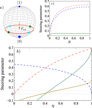
Figure 1. Quantum jump unravelings: (a) Bloch sphere representation for the case  of the steady state
  (brown arrow), and three different K = 2 PREs:
  (dark blue) at the poles, and on the equator
  (dark green), and
  (cyan). For all states, the volume of the sphere represents the corresponding probability
  in the PRE. The red dashed circle show the locus of all the
  s. (b) The value of the steering parameter S (8), versus
  : for
: for  settings at R = 0.01 (brown dotted); and for n = 4 and
  (green solid). For the latter case the first term of the EPR-steering inequality (8) (red dot-dashed), and the second term of (8) (blue dashed), are also shown. (c) displays S and the same ensemble averages as in (b), with the same line styles, as a function of R for efficiency
  . S has maximum value of 0.05 at
  .
.
Download figure:
Standard image High-resolution imageIn [19], the unravelings for PREs were explicitly constructed only for the case of a single output (L = 1). Here we extend that theory by finding explicit unravelings for the above PREs for a two-channel ME. For  it is trivial to see that no LO is required, as
  cause jumps between the
  -eigenstates. For
  we require an adaptive scheme with each
  taking two possible values,
  . Here l, the label for the output channel, also takes the value
  , but that is independent of the
  defining the two values for the LO. The adaptivity required is that every time a detection in either channel occurs, the LO for both channels is swapped from their
  values to the − values, or vice versa. See appendix
  -unravelings that we will design an EPR-steering test that works even with low efficiency.
5. Quantum jumps are more loss-tolerant
For the unit-efficiency case, the z unraveling is such that  for the conditional states (the elements of
  ). If this unraveling were the OPDM of the system then the complementary variable
  (for any
  ) would necessarily have zero mean. However, this operator has a non-zero conditional mean for the PRE
  . Consider a finite set of n different
  values
  , so that, with the z unraveling, Alice has a total of
  unravelings. Then the above, unit-efficiency, considerations suggest the following EPR-steering inequality [22]:
Here ![${{{\mbox{E}}}^{z}}\left[ \bullet \right]$](https://content.cld.iop.org/journals/1367-2630/16/6/063028/revision1/njp495815ieqn105.gif) means the ensemble average under the z unraveling, so that
means the ensemble average under the z unraveling, so that  appearing therein means
 ![${\mbox{Tr}}\left[ \varrho {{\hat{\sigma }}_{z}} \right]$](https://content.cld.iop.org/journals/1367-2630/16/6/063028/revision1/njp495815ieqn107.gif) , where
, where  is the conditional state under that unraveling, and likewise for the
  unravelings. The function f(n) is defined in [22] and asymptotes to
  as
as  .
.
In (8) we are not assuming unit efficiency; the unravelings are as defined above, but the long-time conditional states will not be pure (and will certainly not be just two in number for each unraveling). Our aim is to show that the no-go theorem for inefficient detection, applicable to diffusive unravelings, is not universal, by showing that (8) can be violated for  . To do this we must evaluate the terms on the lhs for the
  different unravelings, although we note that by the symmetry of the problem,
 ![${{{\mbox{E}}}^{\varphi }}[|{{\hat{\sigma }}_{\varphi }}|]$](https://content.cld.iop.org/journals/1367-2630/16/6/063028/revision1/njp495815ieqn114.gif) is independent of
is independent of  . The ensemble average
  can be done semi-analytically, while that for
  requires stochastic simulation; see appendix
  , and varying
  , and for n = 4 and
  .
.
The critical threshold efficiency for jumps to violate (8), is  , which is considerably below the limit of 0.5 necessary for diffusion according to our theorem. This is the second main result of this paper. This
  is achieved in the limits
  and
and  , neither of which are convenient because the first implies that even when there is a violation it will always be very small (compared to the maximum possible violation of unity at
  ), and the second because it requires infinitely many measurement settings. However, we show that a decent violation, of 0.05, is achievable with just n = 4
  settings, for an efficiency
  , which is still significantly below the 50% limit. This was for an optimized value of R, found numerically, of
  .
.
6. Comparison with quantum diffusion
We now consider the same ME (6) and the same EPR-steering inequality (8), applied to diffusive unravelings (2). Here, with  we have
  and the optimal
  unraveling is
  . For diffusive unravelings, there is no unraveling that is particularly useful for Alice to be able to predict Bobʼs value for
  , so for the z unraveling we simply use an arbitrary
  unraveling (this is still better than using no unraveling i.e. replacing the
 ![${{{\mbox{E}}}^{z}}\left[ \bullet \right]$](https://content.cld.iop.org/journals/1367-2630/16/6/063028/revision1/njp495815ieqn135.gif) term by
term by  . Since, as in the jump case,
 ![${{{\mbox{E}}}^{\varphi }}[|{{\hat{\sigma }}_{\varphi }}|]$](https://content.cld.iop.org/journals/1367-2630/16/6/063028/revision1/njp495815ieqn137.gif) is independent of
is independent of  , we only have to simulate one unraveling. This is described in appendix
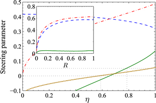
Figure 2. Quantum diffusion unravelings: the value of the steering parameter S (8), versus  : for
: for  settings at R = 0.01 (brown dotted); and for n = 4 and
  (green solid). Also shown are the first and second terms of the EPR-steering inequality (8), both for n = 4 (red dot-dashed and blue dashed, respectively). Inset displays S and the same ensemble averages as in the main figure, with the same line styles, as a function of R for efficiency
  . S has maximum value of 0.05 at
  .
.
Download figure:
Standard image High-resolution imageThe critical efficiency is  , greater than 0.5 as expected, for
  . While this is less than the all-diffusive
  of [10], it is a long way above the quantum jump
  found above. Interestingly, analytical calculations (see appendix
  ,
,  , where
  changes sign at
  . Restricting to n = 4 and looking again for a decent (0.05) violation, we obtain
  at an optimal value of
  .
.
7. Conclusion
In conclusion, we have explored the 'quantumness' of dynamical quantum events by considering their dependence upon distant detectors. For the experimental task of ruling out all OPDM for an open quantum system we have: (i) proven it is impossible to achieve this by diffusive unravelings with efficiencies below 50%; and (ii) exhibited a set of quantum jump unravelings that would allow such a task, for a qubit, with an efficiency as low as  . Moreover, even allowing for a decent margin of error and other experimental realities, a jump efficiency of only
  is required for our system, whereas the corresponding figure for diffusive unravelings is
  . That is, it is far easier to show that the stochasticity of quantum jumps arises in the distant detector (as opposed to being intrinsic to the system) than it is to show this for quantum diffusion, and in that sense the former are more quantum. For future work we believe that it will be possibly to prove even stronger no-go theorems for diffusive unravelings, but also to find even more robust EPR-steering tests. In this context, the recently reported diffusive monitoring efficiency of 49% in superconducting qubit experiments [23, 24], and photon counting efficiency of over 75% in quantum steering tests [25] are encouraging for performing an experimental test in the near future.
Acknowledgements
This research was supported by the ARC Centre of Excellence Grant No. CE110001027. We thank Jay Gambetta for discussions.
Appendix A.: PREs and adaptive monitoring
For a qubit it has been shown that a PRE of the minimum size (K = 2), that is,  , always exists [19]. Moreover, there are as many K = 2 PREs as there are distinct (not necessarily linearly independent) real eigenvectors of the matrix A, which appears in the Bloch equation
  equivalent to
  for the qubit state represented by
  . Therefore, since matrix A in equation (7) of the paper has one real eigenvector in the z direction, it gives rise to a K = 2 PRE, as
  . This A also has infinitely many real eigenvectors in the x–y plane, which we can parametrize by the azimuthal angle
  , giving rise to the K = 2 PREs, as
  .
.
To realize these PREs in the lab, one would require different setups of measurement schemes, and in general these must be adaptive. It is clear that  does not require an adpative scheme, but the
  do. In [19] it was shown how to construct the required scheme for the case of a single output channel. Here we extend that approach to ME (6) with two output channels. What is required is to find pairs of LO amplitudes,
  . Here l labels the output channel, while
  refers to the state of the system prior to the jump, which must reverse sign upon a jump:

Solving this system of equations gives  as given in the paper. Thus to confine the systemsʼs dynamics into the
  it is essential to switch the LO strength for both channels from one sign to the other one, upon a detection in either channel.
Appendix B.: Simulating average values
Appendix. Adaptive detection
Letʼs say system starts at time t = 0 from some arbitrary initial state. Based on the quantum trajectory theory relevant for inefficient detections  , the unnormalized system state matrix
  then evolves according to [17]

where  with
with  the weak LO amplitudes, and
 ![$\mathcal{J}\left[ \hat{a} \right]\bullet =\hat{a}\bullet {{\hat{a}}^{\dagger }}$](https://content.cld.iop.org/journals/1367-2630/16/6/063028/revision1/njp495815ieqn174.gif) . Until the first jump occurs at time
. Until the first jump occurs at time  the systemʼs state is described by the conditional state
 ![$\varrho \left( t \right)=\tilde{\varrho }\left( t \right)/{\mbox{Tr}}\left[ \tilde{\varrho }\left( t \right) \right],$](https://content.cld.iop.org/journals/1367-2630/16/6/063028/revision1/njp495815ieqn176.gif) where
where ![${\mbox{Tr}}\left[ \tilde{\varrho }\left( t \right) \right]$](https://content.cld.iop.org/journals/1367-2630/16/6/063028/revision1/njp495815ieqn177.gif) is the probability of no photon detection for the interval
is the probability of no photon detection for the interval  . We can generate the jump time
  with the correct statistics by generating a random number u uniformly distributed in
 ![$\left[ 0,1 \right]$](https://content.cld.iop.org/journals/1367-2630/16/6/063028/revision1/njp495815ieqn180.gif) , and solving
, and solving ![${\mbox{Tr}}[\tilde{\varrho }({{t}_{1}})]=u$](https://content.cld.iop.org/journals/1367-2630/16/6/063028/revision1/njp495815ieqn181.gif) . Then using a new random number we determine which jump occurs with the relative weights
. Then using a new random number we determine which jump occurs with the relative weights ![${{w}_{\pm }}=\eta {\mbox{Tr}}[\hat{c}{{_{\pm }^{^{\prime} }}^{\dagger }}\hat{c}_{\pm }^{^{\prime} }\varrho ({{t}_{1}})]$](https://content.cld.iop.org/journals/1367-2630/16/6/063028/revision1/njp495815ieqn182.gif) . The new starting state of the system is
. The new starting state of the system is ![$\varrho ^{\prime} \left( {{t}_{1}} \right)=\eta \mathcal{J}\left[ \hat{c}_{\pm }^{^{\prime} } \right]\varrho \left( {{t}_{1}} \right)/{{w}_{\pm }}$](https://content.cld.iop.org/journals/1367-2630/16/6/063028/revision1/njp495815ieqn183.gif) corresponding to the appropriate jump operator. This algorithm is repeated to generate a long sequence of subsequent jumps at times
corresponding to the appropriate jump operator. This algorithm is repeated to generate a long sequence of subsequent jumps at times  , and once the transients have decayed away we can obtain the required ensemble averages as time averages:
Here  is the number of jumps after which system can be taken to have relaxed to the steady state, and
  is the time of each individual jump. We use
  .
.
Appendix. Direct detection
Under direct detection (zero LO), each jump operator  prepares the system in one of the states
  , and this fact enables us to solve for this dynamics without resort to stochastic simulation. Following a jump, the unnormalized system state again smoothly evolves, as in (B.1) but this time without any LO field, that is

Here the conditional state matrix ![$\varrho \left( t \right)=\tilde{\varrho }\left( t \right)/{\mbox{Tr}}\left[ \tilde{\varrho }\left( t \right) \right]$](https://content.cld.iop.org/journals/1367-2630/16/6/063028/revision1/njp495815ieqn190.gif) until the first jump is a mixture of
until the first jump is a mixture of  and
and  . Depending on the initial condition, these states are
 ![${{\tilde{\varrho }}^{\pm }}\left( t \right)=\frac{1}{2}\left[ {{p}^{\pm }}\left( t \right)+{{\tilde{z}}^{\pm }}\left( t \right){{\hat{\sigma }}_{z}} \right]$](https://content.cld.iop.org/journals/1367-2630/16/6/063028/revision1/njp495815ieqn193.gif) , where
, where  and
and  are the solution of the following set of


with the appropriate initial condition of  and
and  .
.
Then the system jumps into either of  with rates
 ![$w_{j}^{\pm }\left( t \right)=\eta {\mbox{Tr}}\left[ \hat{c}_{j}^{\dagger }{{\hat{c}}_{j}}{{\varrho }^{\pm }}\left( t \right) \right]=\eta \left[ 1+j\times {{z}^{\pm }}\left( t \right) \right]/2$](https://content.cld.iop.org/journals/1367-2630/16/6/063028/revision1/njp495815ieqn199.gif) , where
, where  also. This is such that the probability that, when a jump occurs, the system jumps into state
  is
is  and can be obtained by solving

Here  appears as the probability for starting in state
  at some time
  , and
, and  is the probability that, given this starting point, a jump occurs in the interval
  and puts the system into state
  . Averaging over the two possible initial states and all the possible times from one jump to the next, should give
  (i.e. the same function as
  , since nothing distinguishes the first jump from the second in the long-time limit.)
Solving (B.6) analytically gives  . This very simple result cries out for an explanation, and here is the simplest one we can furnish. In the case of efficient detection, the system state is always either
  or
or  , and alternates between them every time a jump occurs. Thus, after every jump it finds itself in either of them with the equal probability of
  . We can model the case of imperfect detection, where both decoherence channels have the same efficiency
  (as we have assumed) as randomly deleting a portion
  of jumps from the full record for perfect efficiency. Since the remaining jumps are an unbiassed sample of the original set of jumps, on average the system state will be equally often in the two states (since the pure post-jump states in the two situations must agree).
The ensemble average we require can be obtained by calculating the below integral
This is directly comparable to (B.2). There the time-average was done by numerically simulating a typical trajectory of jumps. Here can calculate exactly the time-average by using the distribution over the initial state  (immediately following a jump) and the time t until the next jump.
Appendix C.: Simulating averages for diffusive unravellings
The case we are interested in, where  , corresponds to to homodyne detection of both channels, with phase
  . As noted in the main text, the ensemble averages are independent of
  so without loss of generality we can take
  . Then the conditional state of the system evolves according to the following stochastic differential equation

where  are independent real Wiener processes. The state of qubit is confined to y = 0 plane such that at any instant of time it can be identified by a point
  in the Bloch sphere. The evolution of this point is governed by the coupled stochastic differential equations


We simulate these using the Milstein method [26]. Once the transients have decayed away (after several  ) we record data for both x and z, to calculate
 ![${{{\mbox{E}}}^{\varphi }}[|\langle {{\hat{\sigma }}_{\varphi }}\rangle |]={\mbox{E}}[|x|]$](https://content.cld.iop.org/journals/1367-2630/16/6/063028/revision1/njp495815ieqn225.gif) and
and ![${{{\mbox{E}}}^{\varphi }}[\sqrt{1-{{\hat{\sigma }}_{z}}{{|}^{2}}}]={\mbox{E}}\left[ \sqrt{1-{{z}^{2}}} \right]$](https://content.cld.iop.org/journals/1367-2630/16/6/063028/revision1/njp495815ieqn226.gif) as time averages.
as time averages.
Appendix D.: Limit of small R
When  , the conditioned system state under quantum diffusion is almost always near the ground state, and
  . Then (C.2) and (C.3) become, to leading order,


Under this approximation it is easy to find the first two moments of x and z for the system in steady state:


From (D.1) one has a Gaussian distribution for x, which enables us to calculate the first term of the steering parameter, ![${\mbox{E}}\left[ |x| \right]$](https://content.cld.iop.org/journals/1367-2630/16/6/063028/revision1/njp495815ieqn229.gif) . For z, however, the above moments show that a Gaussian cannot be a good approximation for z (because it is bounded below by
. For z, however, the above moments show that a Gaussian cannot be a good approximation for z (because it is bounded below by  ). However, we can consider a Taylor series expansion of
  about
about ![${\mbox{E}}\left[ z \right]$](https://content.cld.iop.org/journals/1367-2630/16/6/063028/revision1/njp495815ieqn232.gif) . This gives the analytic expression of steering parameter for small R as
. This gives the analytic expression of steering parameter for small R as

where  comes from higher-order (beyond second-order) moments of z, which are not negligible (they do not scale with R). Thus, whatever the form of
  , this does not change the scaling with R:

Ignoring  and using
  [22], we predict a critical efficiency, where
  , of
, of  . From the stochastic simulations with R = 0.01, we found (see main text)
  , showing that
  is non-negligible, as expected, but not very important.
Footnotes
- 2
- 3
It is crucial to note that the different detectors, being distant, do not change the coupling of the atom to the electromagnetic field and hence do not change the average evolution of the atom, described by a master equation for its mixed state
 .
.
