


Abstract
Modelling the behaviour of stock markets has been of major interest in the past century. The market can be treated as a network of many investors reacting in accordance to their group behaviour, as manifested by the index and effected by the flow of external information into the system. Here we devise a model that encapsulates the behaviour of stock markets. The model consists of two terms, demonstrating quantitatively the effect of the individual tendency to follow the group and the effect of the individual reaction to the available information. Using the above factors we were able to explain several key features of the stock market: the high correlations between the individual stocks and the index; the Epps effect; the high fluctuating nature of the market, which is similar to real market behaviour. Furthermore, intricate long term phenomena are also described by this model, such as bursts of synchronized average correlation and the dominance of the index as demonstrated through partial correlation.
Export citation and abstract BibTeX RIS

Content from this work may be used under the terms of the Creative Commons Attribution 3.0 licence. Any further distribution of this work must maintain attribution to the author(s) and the title of the work, journal citation and DOI.
GENERAL SCIENTIFIC SUMMARY Introduction and background. Two major features of financial markets are well observed: (1) fluctuating short time returns of individual stocks and of indexes; (2) strong correlations between individual stocks and between stocks and indexes. These features are perceived as the result of an effcient market, where agents react to new information. However, the flow of new information cannot explain the highly fluctuating behaviour of markets, as the rate of new information is relatively low. Recently, advances in financial research indicate the importance of herding on market behaviour, due to human financial interactions and the tendencies of individual investors to be influenced by a group.
Main results. In this article, a simple model that takes into account the above tendencies is proposed. The model was able to capture several key short time features of the market: the autocorrelation of the return; the Epps effect observed in average correlations; the daily return fluctuative nature. In addition, more complex behaviours related to longer time scales were also described by the model, such as the averaged partial correlations of stocks with respect to other stocks and to the index and stocks synchronised high correlation bursts.
Wider implications. The model results indicate the important role of human interactions and herding in generating different stock market phenomena. More thorough analysis, taking into account different stock weighting in the index, and time dependence of the volatility and correlations, will enable the differentiation between the short time herding related phenomena from the long range trends.
 Figure. Bursts of synchronised correlation in the modelled stock market. Each horizontal line represents the dependence of average correlation of one modelled stock on time, where the left y-axis displays the number of the stock. The black curve is the averaged average correlation for all stocks.
1. Introduction
One of the central ideas in economics is that investors take rational decisions in accordance to information in the form of news, sometimes referred to as Homo economicus [1, 2]. This has led to the notion of market efficiency and the hidden assumption that capital markets are dominated by exogenous variables as external pressure and changes in the environment and not by endogenous variables such as human behaviour [3, 4]. However, recent advances in economics and behavioural finance have led to the understanding that in practice, financial markets are not perfectly efficient and the effects of human behaviour on financial markets are gaining more and more attention [3–6].
The importance of human behaviour and its effect on the stock market were recently supported by a novel approach of analysing large scale data regrading financial topics, appearing in the media. These analyses include mood analysis on Twitter [7], search volume analysis on Google [8], article viewing analysis on Wikipedia [9] and even the analysis of financial news [10]. These examples demonstrate the correlation between stock market moves and behavioural trends reflected in various media channels.
A prominent human social behaviour that might have effect on financial decisions made by investors, is the human tendency to belong to a group. A common expression of that behaviour is herding, which is common to many natural systems: ant colonies, fish schooling, bird flocking, animal herding and even bacterial growth [11, 12]. In financial markets this is especially true for analysts and consultants, who trade their customers money. Investors are influenced by the decisions of other investors and most investment managers prefer not to invest contrary to the group [13, 14]. New information is very noisy and not accurate, whereas the group decisions are perceived as better than the individual ones [13–19].
Within this framework, two major features of financial markets are very well known, yet still noteworthy:
- Market prices are highly fluctuating and unpredictable. The short time fluctuations are an order of magnitude larger than the effect of long range drifts.
- Strong collective behaviour in the stock market is identified [13–19]. This collective behaviour is observed in the correlations between the prices of stocks, and in the pronounced correlation between different indexes in different markets [20, 21].
These features are hard to explain as the result of new information. The flow of new information, by itself, is not enough to explain the highly fluctuating behaviour of financial markets [22, 23]. The rate of new substantial information is very low, compared to the market fluctuations rate. In addition, the information is often not clear enough to cause a correlated behaviour.
Following the observations above, a combination of the unpredictable reaction to information and the collective behaviour in markets is necessary when trying to model the market behaviour. Therefore, we propose a simple model that balance between these two characteristics.
The suggested stock market model consists of the coupled dynamics of the market index and several stocks. In the stock market, the index is a good representation of the group activity [24, 25]. Every investor is effected by the actions of other investors, and when making a decision regarding a single transaction, the group behaviour is taken into account. Consequently, the transaction return should be strongly correlated to the change in the index, at the time of the transaction.
In this paper, we present an analysis of the proposed model used to describe the observed short time scale behaviours of financial markets. In section 2, we describe our model and the method used for its calculation and analysis. In section 3 the lagged autocorrelation of the stock returns with different time lags is analysed and compared to empirical data. The Epps effect apparent in the correlations between the modelled stocks is presented in section 4. Section 5 features the analysis of daily results using the suggested model focusing in the fluctuative nature of the daily returns of the index and the stocks. In section 6 long term behaviour of the model is described. Finally, a discussion of the results and a summary of the presented work are brought on section 7.
2. Method
We devise a new stock market model that produces time series of stock returns and their weighted average, the index return.
Let us start with n time series, each representing the return of a certain stock (for example, n = 30 is the number of stocks in the Dow-Jones index). In each time interval the return of each stock is denoted by  , where i and j are the stock and time indexes respectively. The change of the index,
  , for the same interval, is defined as:

Given  for all i and
  it is possible to calculate
  using the correlation between stock i and the index and a random term, based on the rationale presented in section 1:

 stands for the initial correlation between the change in the index and that specific stock. For simplicity it is assumed that
  is constant for all stocks. K is an arbitrary number (of none real qualitative significance. The parameters R and K have a major quantitative significance, though) and r is a random number, distributed so that it represents the reaction of investors to information and their general behaviour. This was done by producing a random number generating function with a tail that decays according to a power law. This function should be constant up to a certain value and decays like
  above that value. Following the procedure presented in [26], the random distribution was chosen to be:

After normalization (i.e.  )
)  and
and  .
.
The term  was used in equation (2) in order to randomly produce the numbers 1 and
  in equal probability multiplying r.
Using the described process,  is calculated and then used to calculate
  and so on for the different stocks. This way, long sequences of
  and
and  are produced.
Remembering that each day is composed of many time intervals, the daily change of the index,  , is calculated as the sum of some consecutive values of
  , where for the next day,
  , it is the sum of the next consecutive time intervals and so on. The term 'daily' is used to describe that each 'day' consists of a specific number of time intervals. The calculated daily return is dimensionless, as it is synthetically constructed. In order to compare it to real market data, gauging or normalization is essential. This will be discussed in section 5. In addition, since stock trading is continuous, the time steps, on which the stock returns are set, are rather artificial. However, the model update rate can be simply seen as a sampling frequency. This way, gauging will also enable us to overcome this artificiality.
3. Lagged autocorrelation
It is reasonable to expect that such an iterative process as presented in the previous section, will produce 'autocorrelated' sequences. An analysis of the correlation of a modelled stock to itself with different time lags was done. Given a time series  , describing the stock return in time, the term
  was calculated (where corr is defined as:
  ) for different values of τ, measured in transactions (or time intervals). We will refer this term as the lagged autocorrelation of
  for time lag τ. Figure 1 presents results obtained for the lagged autocorrelation of an arbitrary stock in a model of 30 stocks, using the parameters R = 0.8 and K = 0.6, running
  transactions. The choice of parameters was such that R, representing the average correlation between the index and any of the stocks, is similar to a nominal value in real markets ranging usually from 0.5 to 0.9 [27]. Naturally, this value changes in time and is also different between different markets and between different stocks within the same market. However, for simplicity, a constant value is used through the whole analysis presented in this paper. The parameter K was chosen so that
  . As previously stated, the choice of parameters has an insignificant qualitative effect, while a thorough investigation of the quantitative significance of these parameters exceeds the scope of this paper.
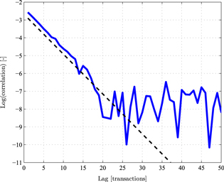
Figure 1. The lagged autocorrelation of a modelled stock. A semi-log plot of the time-lagged correlation of one stock, chosen arbitrarily out of 30 modelled stocks, as a function of the time lag, using R = 0.8 and K = 0.6 for  transactions. The dashed black line is a linear fit of the results for
  .
.
Download figure:
Standard image High-resolution imageThe qualitative picture illustrated in figure 1 is consistent with real market data. The correlation decreases exponentially in time up to some point ( –20 transactions) at which the correlation essentially disappears (it is purely statistical). These results should be compared to those presented in [21, 28, 29], where the same qualitative results are obtained. In addition, by comparing the results to the empirical data, it is possible to add a time scale to the artificial time intervals used. Since in real market data such correlations exist for time lags of up to a few minutes, we can evaluate that for the chosen set of parameters in the model, each time interval or transaction is equivalent to a few seconds. For example, the actual time interval between consecutive announcements of the Dow-Jones index is 2 s [30], 1 s for the DAX index [31] and 15 s for S&P500 [32] and FTSE100 [33].
4. The Epps effect
The Epps effect is a phenomenon described by the decrease of empirical correlation between the returns of two different stocks with the increase of the sampling frequency of the data [34]. Since the description of the effect [34–37], many efforts were made in order to shed more light on the effect and its sources.
Two major factors leading to the effect have been revealed up to now [37–41]:
- Possible lead-lag effect between stock returns, which can appear mainly between stocks of different capitalization or for some functional dependencies between them.
- Asynchronicity of ticks in case of different stocks.
The analysis of empirical data showed that the explanation of the effect solely by any of the factors above is not satisfactory [37, 38]. Using the suggested model, it can be deduced that the explanation for the Epps effect might be different than previously suggested. The proposed factors for the Epps effect are irrelevant in the model, since no direct correlation or functional dependencies exist between the modelled stocks and the possibility of ticks asynchronicity was not taken into account. The correlation between the stocks in the model is only due to their correlation to the index, and the modelled herd behaviour concept.
In figure 2 (a) results of the average of the correlation between the modelled stocks to one specific arbitrary modelled stock are presented.
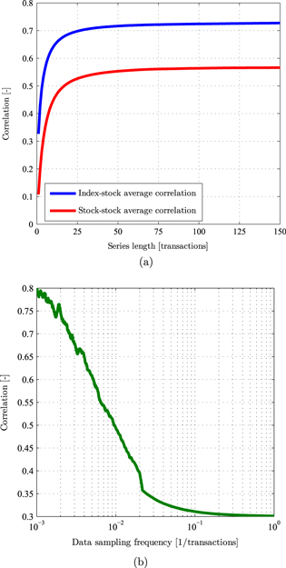
Figure 2. The Epps effect in the modelled stock market. (a) The dependence of  (blue) and
  (red) on m, the sliding window width (or the averaged data series length); (b) the dependence of the averaged correlation between the stocks and the index on f, the sampling frequency of the data, averaged for a window of 50 transactions constant width. The results were obtained for a modelled market with 30 stocks, where R = 0.8 and K = 0.6 and for
  transactions.
Download figure:
Standard image High-resolution imageThe calculation was conducted as follows: a modelled stock market with index and n stocks was produced for  transactions and the parameters used were R = 0.8 and K = 0.6. The resulted time series can be numbered from 0 to n, where
  is the ith stock return time series (the stocks were arbitrarily numbered) and
  is the modelled index return time series. For a given integer m, it is possible to calculate the average values of sliding windows of width m (measured in transactions) of
  , denoted as
  . Using these calculations, the following term can be derived:

 is a measure of the average correlation between the first stock return and the return of the other stocks (stock–stock correlation) for a given sampling frequency. Obviously, increasing the sampling frequency of the data is equivalent to decreasing the sliding window width, m. The results presented in figure 2(a) for
  are clearly consistent with the Epps effect.
The effect is also apparent when taking into account the average correlation between the stock returns and the index return (index–stock correlation), calculated as follows and presented in figure 2(a):

Also calculated was the average correlation between the index and the stocks return for increasing sampling frequency of the data (without averaging over sliding windows of changing widths), as presented in figure 2(b).
From figure 2 it is possible to observe that although the R parameter in the model was 0.8, the average correlation was 0.3, when looking at each transaction separately (large sampling frequency). As the sampling frequency decreases, the average correlation goes closer to 0.8. These results, in which the correlation between pairs of stocks is lower than the correlation between stocks and the index (see figure 2(a)), are consistent with actual observations [24].
Identifying the Epps effect in the model results suggests that the underlying assumptions of the model presented previously might be additional factors to the Epps effect. Thus, it demands further work to be carried out in order to test this conclusion thoroughly.
5. Daily results
The fluctuative nature of the market is a key feature of the market one would expect the suggested model to possess. In order to identify this feature in the model, the distribution of the market return should be analysed.
First, the index return time series ( ) is used to produce the 'daily' return time series of the index. Suppose each day is defined to be consisted of d transactions (in our case d = 780 transactions/day is used, as transaction every 30 s is assumed), it is possible to define the daily return of the index simply by summing over each 'day'. This time series is defined as follows:

where k is the day number.
The modelled index and stocks return series are synthetically created and therefore have no natural scale and can be seen as dimensionless. D, therefore, also lacks a scale and should be normalized in order to be quantitatively compared to any data representing real markets. The choice of normalization was such that the standard deviation of the normalized modelled daily change time series will match the typical standard deviation of daily change time series of leading indexes. It might be seen as a method of adding units to the modelled daily return, as it is naturally dimensionless, while the real index daily change time series are measured in percent.
This normalization was done the following way: the mean value of D ( ) that is relatively close to 0 and its standard deviation (
 ) were calculated. In addition, the daily change time series of each major index taken into account (Dow-Jones, S&P500, NASDAQ, DAX, FTSE100, CAC40, NIKKEI225, Hang Seng, Shanghai stock exchange and Bombay stock exchange) was calculated as well. This was done by taking
  for the daily change in day k of the index I, where
  is the closing price of I in day k measured in points. Each of these time series has a mean value (relatively close to 0) and a standard deviation. When averaging over all ten indexes taken into account the average standard deviation was
  . Therefore, the normalized modelled daily change time series was calculated simply by taking
  , so that
  . Due to the additivity of the daily change (see equation (6)), this implicates that the actual index and stocks returns can be simply normalized by taking
  , where i and j are the stock and time (or transaction) indexes respectively.
Figure 3 presents a typical daily change plot in time. The results were obtained for a modelled market with 30 stocks, where R = 0.8 and K = 0.6 and for 780 transactions a day, reflecting the number of 30 s time intervals in a 6.5 h trading day. The presented results should be compared to those presented in figure 1 in [26].
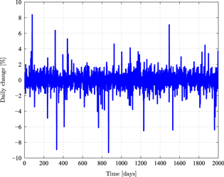
Figure 3. The daily change of the modelled index. The calculation was performed with 30 stocks, where R = 0.8, K = 0.6 and d = 780 transactions/day, taking account of 2000 days. Comparison should be made to figure 1 in [26].
Download figure:
Standard image High-resolution imageFigure 3 shows typical results of the daily return time series for a modelled index. These results resemble results obtained in practice for actual indexes.
Yet another measure of how fluctuative is a modelled index, which can be used to test its resemblance to actual indexes, is the generation of a probability distribution function (pdf) of the daily change (the absolute value of the daily change was taken into account, as the distribution is approximately symmetric) and its comparison to real data. Such a comparison to the daily change probability distribution function of some of the leading indexes was made, and is presented in figure 4. These results were obtained, as previously presented, for a modelled market with 30 stocks, where R = 0.8 and K = 0.6 and for 780 transactions a day, this time taking account of 70 000 days in order to improve the statistical significance of the results. The probability distribution function of the modelled index taken into account is the normalized time series  .
.

Figure 4. The probability distribution function of the absolute daily change. (a) The probability distribution function of the absolute daily change of leading indexes—Dow-Jones (blue), S&P500 (green), NASDAQ (red) and FTSE100 (cyan). Also presented is the probability distribution function of a Lévy stable distribution [42] (dashed black curve) with the parameters  ,
,  ,
,  and
and  ; (b) the probability distribution function of the absolute daily change for the modelled index with 30 stocks, where R = 0.8, K = 0.6 and d = 780 transactions/day, taking account of 70 000 days (magenta curve) and the probability distribution function of a Lévy stable distribution (dashed black curve, the parameters taken were the same as presented in (a)). The light green curve shows the results for the modelled index with 30 stocks where R = 0.8, K = 0.6 and d = 780 transactions/day, taking account of 70 000 days (the same parameters as the magenta curve), where the modelled index was calculated for a normally distributed random number and not power law distributed, meaning equation (2) was taken as
  , where
  .
.
Download figure:
Standard image High-resolution imageBoth qualitatively and quantitatively, a similarity between the modelled index and the actual data is obtained. This resemblance is a good measure for similar fluctuative nature, and the modelled index is therefore close in these characteristics to actual indexes. Also depicted in figure 4 is that the distribution of the daily return both in real markets and in the modelled index approximately follows a Lévy stable distribution [42] (see figure 4(a)), which is known for characterizing many processes in economics and finance in general [43, 44]. While the model provide no explanation for this specific functional dependence of the distribution, the assumptions on which it stands are enough in order to achieve this dependence. Furthermore, the quantitative similarity demonstrates that the nominal values of R and K used, as well as the value of the power law exponent, make sense.
While figure 4(b) demonstrates the high similarity between the model results and real market data, it is clearly seen that as expected, a different choice for the random distribution describing the non-correlated term in the model (see section 2), such as a normal distribution, will fail in describing both qualitatively and quantitatively the fluctuative nature of the market. The normal distribution fails to capture extreme changes, as the distribution tail is short, leading to the rapid decay of the daily change pdf depicted in figure 4(b) (the light green curve). In that sense, the results presented in figure 4 demonstrate that the choice in a power law distribution function in equation (2) makes sense.
Also to be noted is that regardless of the observed similarities between the volatility distribution of the model results and of actual indexes, no temporal order can be obtained using the model, in the sense that exists in indexes [26]. This is, of course, due to the purely randomized method of constructing the modelled index.
6. Long term behaviour
The results presented in the previous sections show how different known behaviours of stock markets can be obtained using the suggested simple model. This success shows that the herding perspective of the driving forces of stock markets is significant and relevant. However, while relatively short term characteristics were obtained, no long term characteristics were analysed using the suggested model in the previous sections.
6.1. Partial correlations
Another market characteristic that be can obtained using the model is the high partial correlations with respect to some stock comparing to the relatively low partial correlations with respect to the index [24]. In order to test this behaviour, a stock market containing 30 stocks was modelled, using the parameters R = 0.8 and K = 0.6. Daily returns were obtained using 780 transactions a day. Given a sliding window of 22 days, the partial correlation of each pair of stocks was calculated, with respect to the index and with respect to two given stocks (arbitrarily chosen) for each window, for consecutive 2000 windows. The results of these calculations are presented in figure 5 .
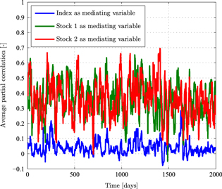
Figure 5. The average partial correlation between pairs of modelled stocks. The calculation was performed with sliding window of 22 days, with 780 transactions a day, 30 stocks, R = 0.8 and K = 0.6. The blue curve was obtained for the modelled index as a mediating variable and the red and green curves were obtained by taking two arbitrary stocks as the mediating variables. Comparison should be made to figure 6 in [26].
Download figure:
Standard image High-resolution imageAs expected, a significant difference was obtained between the average partial correlation of the stocks with respect to an arbitrary stock comparing to the average partial correlation with respect to the index [26]. In accordance with the previous results, the suggested model is found successful in qualitatively and even quantitatively describing known behaviours of the stock market. The results presented in figure 5 of the average partial correlation with respect to the index are very similar to those obtained from real data [45]. However, the small difference that still exists between the modelled and the empirical results might be attributed to the effect of external events that was not taken into account in the model.
6.2. Synchronized correlation
In the previous sections we used the suggested model in order to show that using the underlying assumptions described in section 1 known behaviours of stock markets can be achieved.
We are also able to demonstrate more complex behaviours of the market using our model. One of these behaviours is the synchronized high correlation between stocks or correlation 'bursts' appearing in major markets [25]. This feature is achievable through random calculation using the suggested model. This is done by analysing the daily return of n stocks market (we used n = 30), taking into account 780 transactions a day, using R = 0.8 and K = 0.6. For each stock i, we calculated the correlation between its daily return and any other stock j daily return for a sliding window of 22 days, thus producing a time series of correlations, denoted as  . Following this calculation it is possible to obtain the average correlations time series of i:

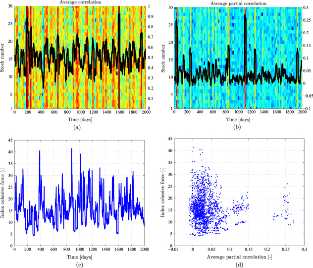
Typical results for  for different stocks in 2000 days are presented in figure 6 (a). The most prominent behaviour depicted in figure 6(a) is the 'synchronized' spikes in the averaged correlation for all stocks, meaning that all stocks show sudden extreme correlation 'bursts' to all other stocks. This result is a known phenomenon [25, 45, 46], and the results presented in figure 6(a) should be compared to those presented in figure 3 in [45], which demonstrate the same behaviour for real leading indexes. Apart from presenting this well known behaviour of the market using the suggested model, it also demonstrates that this result is a partly statistical feature, and not the result of an ordered behaviour of the market as might be hypothesized. As previously stated, no feature or behaviour of the market that involves some sort of temporal order be the result of the suggested model due to its randomized nature.
Figure 6. Bursts of synchronized correlation in the modelled index. (a)  for all n = 30 stocks, calculated using a sliding window of 22 days, 780 transactions per day, R = 0.8 and K = 0.6. Each horizontal line represents the average correlation of one stock, where the left y-axis displays the number of the stock. The black curve is the averaged average correlation for all stocks (
 ); (b)
  for all n = 30 stocks, calculated using a sliding window of 22 days, 780 transactions per day, R = 0.8 and K = 0.6. Each horizontal line represents the average partial correlation of one stock, where the left y-axis displays the number of the stock. The black curve is the averaged average partial correlation for all stocks (
 ); (c) the index cohesive force, calculated using a sliding window of 22 days, 780 transactions per day, R = 0.8 and K = 0.6. The result is the quotient of the averaged average correlation and the averaged average partial correlation with respect to the index; (d) the index cohesive force dependence on the averaged average partial correlation (as calculated in (b) and (c), respectively).
Download figure:
Standard image High-resolution image
A related behaviour is obtained when calculating the average partial correlation using the index as a mediating variable between pairs of stocks (simply replace the correlation between i and j with partial correlation between i, j and the index) and will be denoted as  . These results are presented in figure 6(b). One can easily see that figures 6(a) and (b) complete together the empirical results depicted in figure 1 on [25]. The average correlations and the average partial correlations can be divided for the calculation of the index cohesive force (ICF) [24, 25]. The ICF is a quantitative measure of the cohesive effect the index has on the dynamics of the stock correlations. This refers to the observed effect the index has on stock correlations, where large changes of the index result in higher index–stock correlations [25]. The value of the ICF is the quotient of the averaged average correlations and the averaged average partial correlations, or
  . The model results of the ICF are presented in figures 6(c) and (d).
As previously mentioned, one can easily see that the model results illustrated in figure 6 are very similar to such obtained empirically for different markets [24, 25, 45, 46]. However, while the results featured in the previous sections show similarities between the model results and known empirical results for short term market phenomena, these results capture long term behaviours, while the underlying assumptions are exactly the same. This may lead to the idea that the index effect on the market is a actually a relatively long lasting effect.
7. Summary and discussion
As the 2008 financial crisis brought more attention to the validity of the current economic theories, it should be taken into account that social tendencies of investors might have effect on their financial decisions. Here we devised a new simple model to quantitatively describe some of the short and long term behaviours of real stock markets taking into account this effect.
The model is consisted of numerically constructing time series for the stock market index return and the stock returns. The time series building process involves two terms: the first is a random one, which represents the uncoordinated influence of many economic variables. The complexity of those variables makes them unpredictable and thus expressed in the process by a random number power-law distributed. The second term is a correlation coefficient multiplied by the index return at the time of the transaction, which represents the collective group behaviour of investors.
The use of constant correlation values between the index and the stocks is a simplifying assumption. The probability density function of stock returns is not stationary and correlations between stocks and between stocks and the index change over time. There are findings of an increase of the mean correlation between stocks with increasing absolute returns over time [47]. However, this dependence was not taken into account in the presented model, as it was kept simplified, at this point, based on a few assumptions and a small number of free parameters. The dependence of correlations between stocks and between the index and the stocks on time and return will be treated in future work. In order to take account of this dependence, it is first essential to analyse the dependence of the mean correlation between stocks, used in [47] and the correlation between index return and a specific stock transaction, used in the presented model.
The model was able to capture several key short time features of the market: the lagged autocorrelation in the return for short times (see section 3); the Epps effect of the change in correlations when enlarging the window size (see section 4); the transition to daily time scale and the fluctuative nature of the daily return (see section 5). In addition, more complex behaviours related to longer time scales were also described by the model, such as the averaged partial correlations of stocks with respect to other stocks and the index, and the synchronized high correlation bursts between stocks (see section 6).
These results demonstrate that some aspects of the human behaviour complexity reflected in the stock market can be described using models such as the suggested one. Moreover, it is the herding notion set in the core of the model that allows for these results. The short term lagged autocorrelation, for example, that can be found in stocks and is described by the model cannot be explained through flow or aggregation of information (due to the short time lag between consecutive transactions), but by some kind of herd behaviour. The term herding is associated with emotional behaviour, where the herd follows some leader blindly, without rational criticism and can lead to extreme catastrophes. This notion is in accordance with actual observations that relate many catastrophes in financial markets to endogenous processes in addition to rational processing of new information [48–53]. In addition, the Epps effect, extensively researched and thought of as originated in different factors related to technical aspects of trading and to inherent lagged correlation between stocks, is shown as possibly originated in investors herd behaviour.
The model describes relatively well short term behaviours, but only some long term behaviours can be described. Other behaviours, such as those involving temporal order [26], are naturally impossible to be achieved using this simple model. Nevertheless, following the model results, it can be deduced that such behaviours, as temporal order or other similar long term effects, cannot be explained solely through the postulated assumptions of the suggested model. More specifically, the correlation between stock and index returns, and the fluctuative nature of the return are not sufficient while trying to capture more complex behaviours. It is however demonstrated that any long range analysis, should take into account that short range behaviour can have a long range influence. The suggested model demonstrates such an influence by the qualitative description of the average correlation bursts observed in real markets (see section 6.2). In that sense, this feature can also be attributed to the market herd behaviour. However, these correlation bursts, not being a short term phenomenon, may broaden the sense in which herd behaviour is perceived. While for the short term behaviours, the index can be thought of as reflecting a 'safe choice' for investors, and therefore is responsible for the stocks lagged autocorrelation, such an explanation cannot be given for the long term behaviours.
Establishing the above, more research should be carried out: the introduction of different weights and correlations for different stocks; analysing the significance of parameter choice; testing the model reaction to perturbation in one or more stocks and in the index; taking into account the existence of clusters of stocks; taking into account information that has a specific and direct effect on the market; calculation of the long term influence of the short term behaviour, analysed in this work and so on.
Acknowledgments
We thank Dror Y Kenett for fruitful discussions and for his comments regarding the results. This research has been supported in part by the Tauber Family Foundation and the Maguy-Glass Chair in Physics of Complex System at the Tel-Aviv University.