Imaging the collective excitations of an ultracold gas using statistical correlations

In the last few years, the degree of control of cold atom experiments has increased to an impressive level, from the control of atomic interactions [1] and trapping geometry [2] to the creation and observation of many-body correlated systems [3] or control at the single atom level [4]. To extract quantitative measurements from such experiments one has to analyze a large number of images [5], which are fitted and compared with theoretical models [6]. For instance, mean-field models describe quantum gases at low temperature, including their dynamics, remarkably well [5, 7, 8]. However, these simple models are far from exploiting all the information contained in the images.

This has motivated the development of alternative model-free approaches to analyze the experimental data. For example, with the minimal assumption that the image accurately represents the gas density profile, one can directly compute averaged observables to reveal the gas collective dynamics [9]. It is also quite efficient to represent the signal in the frequency domain, using Fourier transforms, to isolate the system response to a resonant excitation [10–12]. In some situations the noise itself contains a lot of information about the system [13] that can be recovered by studying the correlations within the images [14, 15].

Here we show that a generic method of signal analysis, principal component analysis (PCA) [16], provides a unique tool to extract all the relevant information from cold atom absorption images without having to rely on a specific model. This tool has already been used to perform filtering [17–19], extract the phase in an interferometric signal [20, 21], and identify the main noise sources in an experiment [22]. Recently it has been shown that PCA can be of interest in performing quantum state tomography [23]. As part of multivariate signal analysis methods, PCA is widely used in numerous applications dealing with large amounts of data [16] to extract signals from a noisy background.

The main result of this paper is that PCA can be extended to the study of the elementary excitations of an ultracold atomic gas and allow the direct observation of the system normal modes. Normal modes or Bogoliubov modes of ultracold atomic gases are the elementary low-energy excitations of the system [6, 24, 25]. They provide a unique insight into the system properties. For example they can reveal the collective superfluid behavior of Bose [26] and Fermi [27–29] gases or probe system dimensionality [9, 30]. Recently an analysis of a set of absorption images using time-to-frequency domain transformation [10–12] was used to isolate a few low-energy collective modes and study their damping. Having access to a method for data analysis which extracts the maximum information will be highly relevant for these studies.

This paper is organized as follows: the PCA method for noise filtering is discussed in section 2. We then show in section 3 that PCA enables a precise identification of the system low-energy excitations. To support our analysis of the experimental data, we compare our findings with the results of numerical simulations in section 4. Finally we discuss in section 5 the requirements for applying PCA to cold atom experiments and the possible improvements that may be achieved.

Let us briefly recall how PCA proceeds [16]. More detail (including formulas) is given in appendix A. We start from a particular data set, which in our case is an ensemble of absorption images where the signal is proportional to the integrated atomic density. We first compute the average of the data set and subtract this mean image from all the images, thus obtaining an ensemble of centered images. We then compute the covariance matrix of this ensemble. The diagonal elements of the covariance matrix contain the variance of the pixels, and off-diagonal elements quantify correlations between pixels. By diagonalizing this matrix we recover the eigenvectors, called principal components (PCs), which are thus uncorrelated. This statistical independence ensures that uncorrelated noise sources are associated with different principal components [16].

Our experiment is described in detail in reference [31]. Briefly, we produce a quantum degenerate gas of ⁸⁷Rb atoms confined in a radio-frequency (rf) dressed magnetic quadrupole trap. We can dynamically control the precise trap shape by varying the magnetic or rf fields, which results in selective excitations of the gas normal modes [30, 31]. We measure the gas properties by performing in situ absorption imaging along the strongly trapped vertical direction. The peak optical density is kept below 6 by repumping only a small fraction of the cloud from the F = 1 hyperfine ground state to the cycling transition. We carefully calibrate the imaging system following reference [32]. The gases we consider in this paper are in the quasi two-dimensional regime: the excitations along the imaging axis are frozen and the dynamics occur only in the horizontal plane. In this plane the system is well described by a harmonic oscillator [31]. We apply PCA to the study of the mode dynamics in an anisotropic quasi two-dimensional gas ($\mu /(\hbar {{\omega }_{z}})\sim 1.5$) with ${{\omega }_{x}}=2\pi \times 33\;{\rm Hz}$ and ${{\omega }_{y}}=2\pi \times 44\;{\rm Hz}$.

As an example of application, figure 1 displays the outcome of PCA applied to 27 images acquired in the same conditions. Due to variations of the stray light during image acquisition, fluctuations of atom number in the experiment, or mechanical vibrations, the images are not exactly identical. The PCA decomposition identifies all these sources of noise, and we can identify them with a principal component: figure 1(c) probably accounts for atom number fluctuations, whereas figures 1(b) and (d) indicate a small jitter of the camera position [17, 22]. Higher-order components (see figures 1(e) through (h)), reflect the presence of diffraction fringes on the probe beam intensity profile. For each of these components, the corresponding eigenvalue accounts for the fraction of the total variance due to the associated noise source.

Zoom In Zoom Out Reset image size

Conversely, when the data set results from the variation of a parameter, PCA allows us to probe the sensitivity of the system to this parameter. In particular, if the system is initially excited and evolves, measurements taken at different times allow us to recover this variation as a principal component. In this paper, we exploit this possibility to directly measure the normal modes of a quantum degenerate gas confined in a harmonic trap.

We make use of our highly versatile trap potential to simultaneously excite several low-energy eigenmodes of the gas. Namely, we displace the trap minimum, rotate the trap axes, and slightly change the trap frequencies. In the new trap the gas is strongly out of equilibrium, and we record its evolution by taking images for different holding times in the trap, covering a time span of 100 ms. Figure 2 shows the result of PCA for this data set (133 images). Compared with figure 1 we see that the principal components have changed.

Zoom In Zoom Out Reset image size

Let us now identify the first principal components. The first two PCs (see figures 2(b) and (c)) display a two-lobe pattern oriented respectively along the columns and the rows of the images: this is characteristic of a dipole oscillation of the cloud. This center of mass motion is due to the trap minimum displacement during the excitation process. The third PC (see figure 2(d)) indicates a global variation of the signal over the whole cloud, which can be interpreted as atom number fluctuations in the experiment. Some of these fluctuations occur because the lifetime in the trap is limited and atoms are lost as the holding time increases¹ . The fourth PC (see figure 2(e)) possesses a striking spatial pattern with four lobes, characteristic of a scissors excitation [33]. Note that the lobes are oriented at 45° with respect to the trap axes (aligned with the first two PCs) as expected. The next two PCs (see figures 2(f) and (g)) look like compression modes of the gas, with a density depletion at the center of the cloud and a correlated augmentation of the density at the sides of the cloud.

The PCs are presented by decreasing eigenvalue, meaning that they account for fewer and fewer variations in the original data set. For this particular experiment the center of mass oscillation is the dominant excitation in the cloud, followed by the response to the rotation of the trap axis and marginally by the compression of the trap. In another experiment (not shown) where the trap rotation was not performed we have verified that no PC displayed the spatial pattern of a scissors excitation.

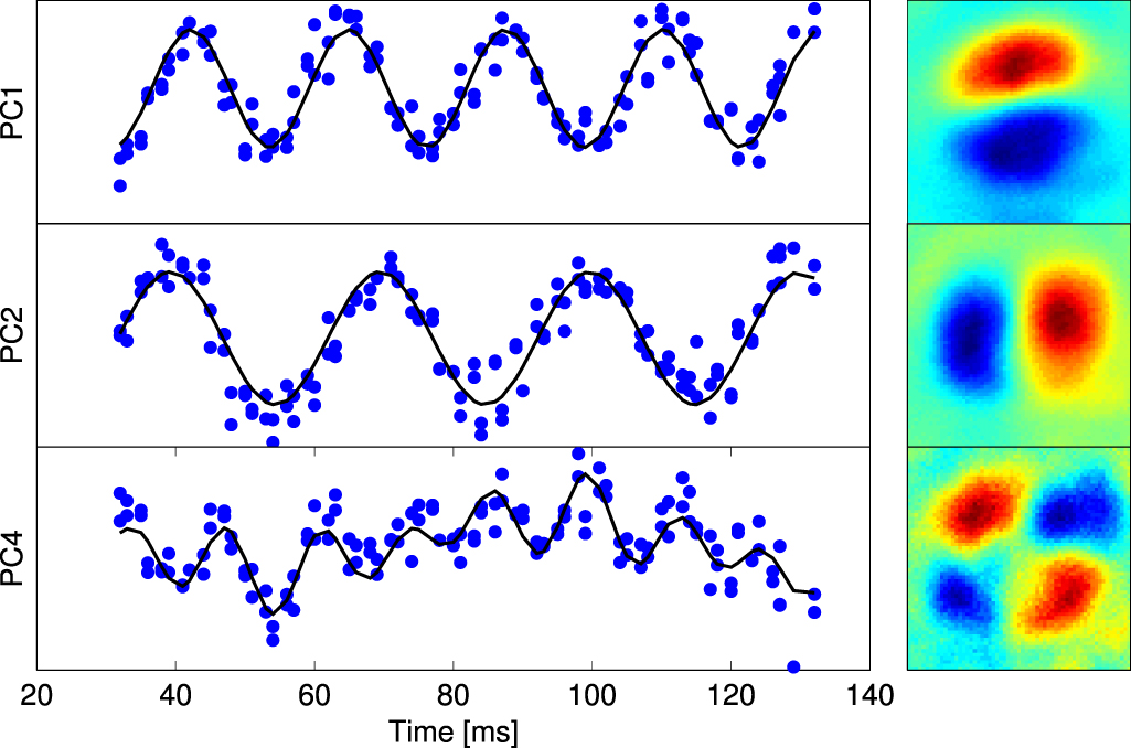
This analysis of the PCs is supported by the study of the time-dependent oscillations of the associated weights, computed by projecting the centered original data set on to the PCs. The result of this computation is displayed in figure 3 for the dipoles and scissors components. Let us focus first on the first two weights: they exhibit sinusoidal oscillations at the expected trap frequencies (44 Hz and 33 Hz). This supports the fact that PCA has correctly identified, as independent components, the center of mass motion of the cloud along the trap axes. The scissors component displays a more complex oscillation pattern. We find that the best fit to the data is given by a sum of three sinusoids, at frequencies 12 Hz, 55 Hz, and 77 Hz. This is related to the fact that the scissors component found by PCA is sensitive both to the collective response of the superfluid part and to the collisionless oscillations of the normal part of the gas [33]. The simultaneous presence of these three frequencies has been evidenced in a three-dimensional Bose–Einstein condensate [34] where simultaneous measurement of the superfluid and normal part of the cloud rotations was obtained by a bimodal distribution fit to the density profiles. Here we note that the same PC gives access to both the superfluid and the normal response to the rotation of the trap axes, which might be used to measure their relative amplitudes.

Zoom In Zoom Out Reset image size

Let us stress that the PCA is able to separate the contributions of the different modes in a given experiment, which may help to design better excitation patterns or focus on higher-order modes [11]. In particular, being able to measure the dipole mode frequencies in the same data set gives access to the natural system clock [24]. Therefore, PCA gives access to direct comparison between measured frequencies and predictions. Moreover, for the data set used in figure 2, we find that the simple hydrodynamic models of references [7, 8] fail to extract these frequencies present in the oscillation of the density, probably due to the fact that several collective modes are simultaneously excited. In this case it is really essential to use a model-free approach to analyze the data set.

We pursue our investigation numerically to compare the principal components with normal modes. We use a zero temperature two-dimensional mean-field model of our cloud and perform a numerical time-dependent simulation which mimics the experimental sequence. We then extract the simulated density profiles using a regular time sampling, thus obtaining a data set of 152 computed images. We finally compare the PCA of this data set with the actual normal modes of the trap, computed using the Bogoliubov–de Gennes equations. Details of the simulations are given in appendix B.

Figure 4 displays the result of the simulations. Let us first focus on the output of PCA (left panel): the first few PCs are like those of figure 2 except for the atom number fluctuations, which are not taken into account in the simulation. In particular, dipole, scissors, monopole-like, and quadrupole-like patterns are present (see respectively figures 4(b) through (f)).

Zoom In Zoom Out Reset image size

This interpretation is supported by the display of the normal modes (right panel), and in particular by the density profiles of figures 4(n)–(q) and (v). To compare these profiles quantitatively, we compute the scalar product between the principal component and the eigenmode images. We find a high degree of overlap for the largest five principal components (dipoles: 99.7% and 99.4%, scissors: 98.5%, monopole-like: 98.8%, and quadrupole-like: 89.2%) when projected onto the corresponding eigenmode. This supports the idea that the largest principal components can indeed be identified with a well-defined normal mode (see also appendix C).

To confirm this result, we compare the oscillation frequency of the principal components (obtained by fitting a sinusoidal function to the time-dependent weight of the simulated density profiles) ${{\omega }_{{\rm pca}}}$ with the frequency of the mode given by the Bogoliubov–de Gennes equations ${{\omega }_{{\rm diag}}}$ and with an analytic hydrodynamical model ${{\omega }_{{\rm th}}}$ [24]. The results obtained with the data of figure 4 are reported in table 1. We find that for the largest principal components the simple sinusoidal behavior correctly fits the data and gives a value compatible with the Bogoliubov–de Gennes theory, within the numerical uncertainty² .

Table 1.  Comparison of the first principal component oscillation frequency ${{\omega }_{{\rm pca}}}$ with the Bogoliubov mode frequency ${{\omega }_{{\rm diag}}}$ and a hydrodynamic Thomas–Fermi model ${{\omega }_{{\rm th}}}$. All frequencies are given in units of the smallest dipole frequency ${{\omega }_{x}}$.

Label	${{\omega }_{{\rm pca}}}$	${{\omega }_{{\rm diag}}}$	${{\omega }_{{\rm th}}}$
Dipole (x)	0.999	0.998	1
Dipole (y)	1.332	1.332	1.334
Quadrupole	1.547	1.552	1.548
Scissors	1.674	1.674	1.667
Monopole	2.441	2.438	2.438

For the collective modes, we expect the correct value for the mode frequency to be given by the diagonalization procedure, as the hydrodynamical model is only approximate. There is excellent agreement between ${{\omega }_{{\rm pca}}}$ and ${{\omega }_{{\rm diag}}}$ for the values reported in table 1, thus validating our experimental findings. However, this is not true for the principal components with a small variance, which exhibit complex temporal behaviors. We observe that these components do not have a significant overlap with one of the modes: PCA is not able to identify them.

We conclude from this example that PCA provides a robust way of evidencing the dominantly excited modes in an out-of-equilibrium ultracold gas. Once the relevant components are isolated, PCA allows us to extract the mode time dependence without having to rely on a model for the atomic response.

We now discuss the requirements for PCA to be efficient and compare it with Fourier analysis. PCA is a statistical method: the data set has to span a sufficiently large number of configurations for the correlations between two different normal modes to average to zero. In particular, to resolve two different modes with close frequencies, the total acquisition time has to be larger than the beat note period. However, it is not necessary to use an even sampling during this time period. In addition, if the populations in the two excitations are very different, resulting in very different contributions to the variance, PCA separates them efficiently, even for shorter observation times; see the discussion in appendix C.

Fourier transformation methods can also be quite efficient for identifying collective modes [10–12]. However, they come with stronger constraints: the time sampling must be regular and the total time should be a multiple of the signal time period. This supposes a priori knowledge of the signal frequency, which may have to be determined iteratively. Moreover, the Fourier transform gives access only to frequencies that are multiples of a fundamental frequency, which complicates the analysis for systems with multiple excitations (see supplementary data at stacks.iop.org/njp/16/122001/mmedia). Finally, a white noise contributes to each Fourier component, whereas it is naturally filtered out in PCA. PCA is not subject to such constraints: if we reduce the size of the data set used in section 4, for example by keeping only one image out of ten, PCA is still able to distinguish PCs close to the excited eigenmodes (dipoles, scissors, and monopole-like with 95% fidelity, but the quadrupole-like component is absent; see supplementary data), even if the Nyquist–Shannon sampling theorem is not verified any longer³ . In that sense PCA is more efficient than Fourier methods.

In conclusion we have shown that, beyond noise filtering [17–19], PCA provides a powerful statistical tool to analyze experimental as well as numerical data sets. When applied to time-dependent systems, it allows for a model-free discrimination of the normal modes and for the measurement of their populations and frequencies. We expect PCA to be particularly relevant for the study of samples where fluctuations play a major role in the physics. Examples include the random creation of defects in the Kibble Zurek mechanism [35] or the correlations between vortices and anti-vortices in a two-dimensional superfluid [36]. We note that PCA is a very general method and would be suitable for other systems with time-dependent signals. In cavity polariton quantum gases, where images can be taken in real time, PCA would allow one to extract the relevant information inside a large data set [37]. Finally, cold trapped ions systems behave as crystals supporting many collective modes, which could be studied using PCA [38].

We envision that PCA is suited to perform Bogoliubov spectroscopy, in the spirit of the method used in references [10, 11]. A mode largely excited by a resonant excitation will be easily identified by PCA and its frequency precisely determined by measuring its eigenvalue with respect to the modulation frequency. In contrast with Fourier methods, PCA can identify the dominantly excited mode using samples covering only one oscillation period of the mode either by recording the time evolution or by varying the excitation phase. This property should prove useful in particular to study over-damped modes.

LPL is UMR 7538 of CNRS and Paris 13 University. We acknowledge helpful discussions with Aurlien Perrin.

We provide here a short recipe to apply PCA to the analysis of density profiles. Other examples of applications are given in references [16, 17]. We stress that the mathematical formalism is quite simple and that most data analysis software provides standard implementation of PCA. We are interested in density profile images and assume that the pixels of each image are stored (row-wise) in a single vector. The first step is to center the data set by computing the average image and subtract it from each image. The entire data set can then be stored in an N × P matrix, denoted B, where N is the number of images and P is the number of pixels. Thus ${{B}_{i,j}}$ contains the jth pixel of the centered image i.

Next we want to compute the eigenvalues of the covariance matrix $S={{B}^{T}}B/(N-1)$ where B^T is the transpose of matrix B. This P × P matrix is in general quite large, so it is hard to diagonalize it directly. However, it is quite simple to show that its rank is at most N. Indeed, assuming that X is an eigenvector of S with eigenvalue λ (meaning $SX=\lambda X$), it is straightforward to verify that Y = BX is an eigenvector of the square N × N symmetric matrix $\Sigma =B{{B}^{T}}/(N-1)$ with the same eigenvalue λ. Therefore, S and Σ have the same spectrum, of at most N real eigenvalues. Knowing an eigenvector Y of Σ, the corresponding eigenvector of S is simply $X={{B}^{T}}Y$. Finally let us stress that these vectors are orthogonal since the S matrix is real and symmetric. We define the associated PCs by normalizing the eigenvectors to unity. In the case of both a large number of pixels and a large number of images the diagonalization of S and Σ is hard to compute. However, since we are a priori only interested in the PCs with the largest variance, they can be efficiently computed by iterative methods [39].

The PCs provide an orthonormal basis spanning the subspace of the data set, and therefore each original image can be represented as a sum of the mean image and the weighted contributions from each principal component. These weights are obtained by projecting the centered image onto the corresponding principal component. By selecting only relevant principal components, the noise can be partially filtered out of the reconstructed images [16].

We model our system by a zero temperature bi-dimensional Gross–Pitaevskii equation:

$$\begin{eqnarray}&&\imath \frac{\partial }{\partial t}\psi =\left( -\frac{{{\nabla }^{2}}}{2}+V(x,y)+{{g}_{2D}}N{{\left| \psi \right|}^{2}} \right)\psi ,\end{eqnarray} \tag{ B.1 }$$

where t is expressed in units of $\omega _{x}^{-1}$, x and y in units of ${{a}_{x}}=\sqrt{\hbar /(M{{\omega }_{x}})}$, and $\psi \equiv \psi (x,y,t)$ in units of $a_{x}^{-1}$. M is the atomic mass, N the number of atoms, and ${{g}_{2D}}=\sqrt{8\pi }a/{{a}_{z}}$ is the reduced coupling constant, where a is the contact interaction scattering length and ${{a}_{z}}=\sqrt{\hbar /(M{{\omega }_{z}})}$ is the size of the vertical harmonic oscillator ground state. The potential reads:

$$\begin{eqnarray}&&V(x+{{x}_{0}},y+{{y}_{0}})=\alpha \frac{{{\left( x{\rm cos} \left[ \theta \right]+y{\rm sin} \left[ \theta \right] \right)}^{2}}+\epsilon {{\left( x{\rm sin} \left[ \theta \right]-y{\rm cos} \left[ \theta \right] \right)}^{2}}}{2},\end{eqnarray} \tag{ B.2 }$$

where $\epsilon =\omega _{y}^{2}/\omega _{x}^{2}$ quantifies the trap in plane anisotropy and the arbitrary angle θ allows us to rotate the trap axes. The auxiliary parameters x₀, y₀, and α can be used to induce a trap displacement and compression. table B1 details the value of the parameters appearing in (B.2) before and after the excitation.

Table B1.  Value of the trapping potential parameters used in the simulation before and after the excitation.

	α		x0	y0	θ
Initial	0.95	1.68	0.5	0.25	10$^{{}^\circ }$
Final	1	1.78	0	0	0$^{{}^\circ }$

The numerical wave function is represented on a square 128 × 128 grid with an equivalent full width of 15a_x in both the x and y directions. For the computations we used ${{g}_{2D}}N=1000$, matched to the experimental conditions.

We use this model to compare the outcome of two numerical computations. On the one hand we mimic the experiment described in section 3 by a) computing the system ground state for the initial potential using an imaginary time evolution algorithm, b) using this result as the input of a real-time evolution in the final potential, and c) performing PCA on regularly sampled density profiles during the evolution. The evolution algorithm relies on a time splitting spectral method, from t = 0 to t = 37.7 (in dimensionless units, corresponding to six periods of the weakest trap axis) using a time step of 10⁻³. The total time is chosen to be close to a multiple of both dipole mode oscillation periods (six periods and eight periods respectively); this ensures that the average density profile computed in PCA is not skewed. The sampling is performed every T_s = 0.126. The result of this procedure is shown in the left panel of figure 4.

On the other hand, we directly compute the small excitation spectrum using Bogoliubov–de Gennes equations obtained from the linearization of (B.1) around the system ground state in the final trap. This implies the ability to diagonalize a square 2¹⁵ × 2¹⁵ matrix, which is quite challenging. Fortunately this matrix is sparse and we are interested only in the lowest-energy part of the spectrum, which means we do not have to compute all the eigenstates. We designed a fast custom C program that uses a combination of an iterative method [39] with an efficient sparse matrix library [40] to compute the relevant eigenvectors. The result of this procedure is displayed in the right panel of figure 4.

We have shown that PCA is very efficient at identifying the normal modes of an excited ultracold gas. This may be surprising but can be understood in the framework of small excitations. Using a hydrodynamic model [24], the gas out-of-equilibrium density profile may be expanded as $\rho ({\boldsymbol{r}} ,t)={{\rho }_{0}}({\boldsymbol{r}} )+{{\sum }_{k}}{{c}_{k}}{\rm cos} \left[ {{\omega }_{k}}t+{{\phi }_{k}} \right]{{f}_{k}}({\boldsymbol{r}} )$, where k labels the normal mode of frequency ${{\omega }_{k}}$, ${{f}_{k}}({\boldsymbol{r}} )$ describes the mode normalized density profile, and c_k is related to the mode population.

In the experiment we observe the gas only at discrete times ${{\{{{t}_{n}}\}}_{n\in [1,N]}}$ and positions ${{\{{{{\boldsymbol{r}} }_{i}}\}}_{i\in [1,P]}}$, and therefore we can write the ith pixel of the nth image as $\rho ({{{\boldsymbol{r}} }_{i}},{{t}_{n}})={{\rho }_{0}}({{{\boldsymbol{r}} }_{i}})+{{\sum }_{k}}{{c}_{k}}{\rm cos} \left[ {{\omega }_{k}}{{t}_{n}}+{{\phi }_{k}} \right]{{f}_{k}}({{{\boldsymbol{r}} }_{i}})+\varepsilon ({{{\boldsymbol{r}} }_{i}},{{t}_{n}})$, where we added a pixel and time-dependent noise contribution $\varepsilon ({{{\boldsymbol{r}} }_{i}},{{t}_{n}})$. PCA starts with the evaluation of the centered data set by averaging over the sampling times $\{{{t}_{n}}\}$: ${{B}_{n,i}}={{\sum }_{k}}{{c}_{k}}{\rm cos} \left[ {{\omega }_{k}}{{t}_{n}}+{{\phi }_{k}} \right]{{f}_{k}}({{{\boldsymbol{r}} }_{i}})$ $+\;\varepsilon ({{{\boldsymbol{r}} }_{i}},{{t}_{n}})+\delta ({{{\boldsymbol{r}} }_{i}})$, where the $\delta ({{{\boldsymbol{r}} }_{i}})$ term is close to zero for a total sampling time $T\gg {{({\rm mi}{{{\rm n}}_{k}}{{\omega }_{k}})}^{-1}}$.

Then the S matrix elements can be written as:

$$\begin{eqnarray}&&{{S}_{i,j}}=\frac{N}{2(N-1)}\mathop{\sum }\limits_{k}c_{k}^{2}{{f}_{k}}({{{\boldsymbol{r}} }_{i}}){{f}_{k}}({{{\boldsymbol{r}} }_{j}})+\Delta ({{{\boldsymbol{r}} }_{i}},{{{\boldsymbol{r}} }_{j}}),\end{eqnarray} \tag{ C.1 }$$

where the term $\Delta ({{{\boldsymbol{r}} }_{i}},{{{\boldsymbol{r}} }_{j}})$ is the effective noise covariance between pixels i and j, due to the initial noise distribution and finite sampling size induced errors. Provided the $\Delta ({{{\boldsymbol{r}} }_{i}},{{{\boldsymbol{r}} }_{j}})$ term is small enough, it is straightforward to verify that the principal components of matrix S are the vectors ${{\{{{f}_{k}}({{{\boldsymbol{r}} }_{i}})\}}_{i}}$, with eigenvalue $\sim c_{k}^{2}/2$. In particular this is true for $T\gg {{\left( {{{\rm min} }_{k\ne {{k}^{\prime }}}}|{{\omega }_{k}}-{{\omega }_{{{k}^{\prime }}}}| \right)}^{-1}}.$ This constraint on T is more stringent than the previous one, especially when two normal modes are close to degeneracy. However, if these two modes have small populations, they make a small contribution to the $\Delta ({{{\boldsymbol{r}} }_{i}},{{{\boldsymbol{r}} }_{j}})$ term.

The conclusion of this analysis is twofold. On the one hand, PCA correctly identifies the most excited⁴ eigenmodes of the system. On the other hand, the total time sampling should be large enough to resolve the beat note between these modes. For practical purposes we empirically found that taking T equal to one beat note period is sufficient; see, for example, figure 3.