


Abstract
Hybrid photonic nanostructures allow the engineering of novel interesting states of light. One recent example is topological photonic crystals where a nontrivial Berry phase of the photonic band structure gives rise to topologically protected unidirectionally-propagating (chiral) edge states of photons. Here we demonstrate that by coupling an array of emitters to the chiral photonic edge state one can create strongly correlated states of photons in a highly controllable way. These are topologically protected and have a number of remarkable universal properties: the outcome of scattering does not depend on the positions of emitters and is given only by universal numbers, the zeroes of Laguerre polynomials; two-photon correlation functions manifest a well-pronounced even–odd effect with respect to the number of emitters; and the result of scattering is robust with respect to fluctuations in the emitters' transition frequencies.
Export citation and abstract BibTeX RIS

Content from this work may be used under the terms of the Creative Commons Attribution 3.0 licence. Any further distribution of this work must maintain attribution to the author(s) and the title of the work, journal citation and DOI.
1. Introduction
Light–matter interaction surrounds us everywhere in nature, and it has played a tremendous role in the development of current technology. Until recent decades it was sufficient to deal with this interaction on average, with many photons and many atoms involved. However, the increasing miniaturization of basic constituents toward nanoscale is a common trend in modern technology. Downscaling to single-atom and/or single-photon levels promotes some traditionally classical research areas into the quantum realm [1–4]. A quantum control over the light–matter interaction will eventually become a vital ingredient of emerging quantum devices, and it is equally important for the development of several related fields, including communication, signal processing, ultrafast optics, optomechanical cooling, imaging and spectroscopy, and quantum information [5]. However, efficient manipulation and control requires a relatively strong interaction at the level of a single atom or a single photon [6–12]. This presents a significant challenge, since the typical interaction scale for individual particles is given by the smallness of the QED coupling constant  . Two possible ways to overcome this natural limitation, and to increase the effects of correlations, are either to use artificial materials and devices, or to resort to many-body effects to produce nonlinearities.
Recent experimental progress in fabricating few-photon sources coupled to one-dimensional (1D) transmission lines [13–20] opens an avenue for creating and manipulating strongly correlated states of photons. It has also triggered a significant number of theoretical studies [21–27]. Our experience from condensed matter and atomic physics teaches us that combined effects of reduced dimensionality and interactions can often effectively enhance correlations, and eventually lead to new collective states of matter with properties which are very different from those of the individual particles (e.g., Luttinger liquids in 1D). This insight is one of the driving forces behind the quest for novel correlated states of photons [28–30].
A different class of collective phenomena is the topological insulating/superconducting state of matter. This state has been recently experimentally realized for electrons [31] and extensively studied theoretically [32]. The main signature of topological properties in the band structure of bulk materials is the existence of edge states, which are insensitive to local perturbations, impurities, or geometrical imperfections. In some—chiral—instances edge states propagate unidirectionally. Recently, the existence of chiral states in photonic systems has been theoretically predicted [33] and experimentally observed [34–39]. These edge states represent an optical analogue of the quantum Hall edge states, and they are characterized by a nontrivial Chern number [40].
In this paper, we suggest the use of 1D unidirectional edge states as a robust platform for the controllable generation of strongly correlated states of photons. To achieve this goal, we couple an array of emitters to a chiral edge state, see figure 1. Experimentally available novel hybrid photonic systems [41] can be used to realize this setup. Photons in the edge channel, populated by an external few-photon source, interact with an ensemble of emitters and produce outgoing states with robust, controllable, and universal properties originating from the topological nature of the edge state. In particular, we find that the outgoing photonic wavefunction does not contain any information about the positions of emitters; its nodes are rather determined by universal numbers—the zeroes of Laguerre polynomials. An initial single-photon wavepacket is fragmented into pieces between these nodes. In the case of two-photon scattering, we observe a clearly pronounced parity effect with respect to the number of emitters, which manifests in a transition from photons' bunching to antibunching as one changes the parity of the number of emitters from even to odd. We also show that the observed properties are robust with respect to fluctuations in the emitters' transition frequencies. The proposed setup can be experimentally realized in the GHz and optical domains with existing nanophotonic elements.

Figure 1. The chiral edge state of a topological photonic crystal. A schematic view of the proposed setup to generate strongly correlated states of photons: the topological photonic insulator (left) possesses a topologically nontrivial band structure (right). If the total Chern number of the bands below the gap is 1, a boundary state inside the gap is formed (its dispersion is denoted by the red line in the right picture). This state corresponds to the chiral edge state of unidirectionally propagating photons (thick red line at the boundary of the photonic crystal). We suggest to embed emitters of an arbitrary level structure (here with two levels) into the edge channel. A population of the edge states by an external few-photon source (in-state) and their propagation through the array of emitters create strongly correlated outgoing photonic states (out-state).
Download figure:
Standard image High-resolution image2. 1D edge modes interacting with emitters
We consider topologically protected states propagating unidirectionally at the edge of the topological photonic crystal. We propose to embed an array of two-level (in general—multi-level) systems—called emitters—into the chiral edge channel. We assume that the transition frequencies of emitters are commensurate with the frequency of the propagating chiral mode of light. Assuming also that the excited emitter states mainly decay into the 1D mode (with a decay rate  ), we note that there are several sources of inevitable losses. Namely, the excited emitter can decay into the continuum of three-dimensional modes in ambient space (with a decay rate Γ0), into the bulk modes of a 2D photonic crystal (decay rate
  ), or to its impurity (bound) states (decay rate
  ). Here we note that the decay into the two-dimensional bulk modes of a photonic crystal is suppressed,
  , since their density of states is zero in the bulk bandgap. We also assume that a 2D photonic crystal is clean enough to neglect the coupling of edge states to eventual mid-gap impurity states.
To generate well-defined chiral modes, it is necessary to minimize losses occurring at the rate Γ0. The waveguide Purcell factor [42]

must then considerably exceed unity, which defines the strong coupling regime. In this expression  is the minimal cross-sectional area to confine the light in vacuum (for the lightʼs wavelength λ0);
  d is the dielectric constant of the host medium where the emitter is embedded; vg is the group velocity of the propagating edge mode. The cross-sectional area
  of the effective confinement is estimated by
  , where b is the thickness of the slab, and
  is the localization depth of the edge mode, B being the bulk bandgap. Thus, the waveguide Purcell factor (1) can be enhanced in three different ways: (1) by reducing the thickness b of the slab; (2) by increasing the bandgap B; and (3) by reducing the group velocity vg. All these methods to achieve the strong coupling regime have been successfully applied in plasmonic nanowires [24, 43, 44] and in the Floquet photonic topological insulators made of helical waveguides [39].
Deep inside the bulk bandgap we can model the dispersion of the chiral edge mode by a linear dependence. In the following we measure all gauge-dependent energy scales from the spectrum linearization point. In the strong coupling regime we neglect losses into the three-dimensional continuum, and consider only the interaction of the edge mode with an array of M emitters. Emitters are modeled by two-level systems with transition frequencies Δa and couplings  , and are placed at different positions xa, which are separated from each by distances larger than the lightʼs wavelength (an arrangement opposite to Dickeʼs [45]). Thus, the Hamiltonian of our model reads
where we use units such that  . The chiral field operators
  satisfy the standard commutation relations
 ![$[a(x),{{a}^{\dagger }}(x^{\prime} )]=\delta (x-x^{\prime} )$](https://content.cld.iop.org/journals/1367-2630/16/11/113030/revision1/njp503555ieqn13.gif) . Transitions between emitters' states are described by the operators
. Transitions between emitters' states are described by the operators  , which satisfy the standard spin algebra
 ![$[S_{a}^{z},S_{a^{\prime} }^{\pm }]=\pm S_{a}^{\pm }{{\delta }_{aa^{\prime} }}$](https://content.cld.iop.org/journals/1367-2630/16/11/113030/revision1/njp503555ieqn16.gif) ,
, ![$[S_{a}^{+},S_{a^{\prime} }^{-}]=2S_{a}^{z}{{\delta }_{aa^{\prime} }}$](https://content.cld.iop.org/journals/1367-2630/16/11/113030/revision1/njp503555ieqn17.gif) . Spontaneous emission to other modes out of the 1D waveguide is modeled by attributing an imaginary part
. Spontaneous emission to other modes out of the 1D waveguide is modeled by attributing an imaginary part  to the transition frequencies
  , in the spirit of the quantum jump picture [46].
The problem is further specified by an initial state. Inspired by experimental realizations of waveguides coupled to emitters [18, 19], we assume that the edge states are populated by an external few-photon source, while emitters are initially prepared in the ground state. Injected photons propagate unidirectionally and interact with an ensemble of emitters, and after a sufficiently long time a stationary state is eventually established: emitters typically relax back to the ground state, while the photonic wavefunction is modified. The evolution of the N-photon wavefunction is described in terms of the scattering matrix  depending on the sets on all transition frequencies Δa and couplings κa

where  and
and  are envelope functions of outgoing and incoming states depending on sets of outgoing
  and incoming
  photonic energies, respectively, obeying the energy conservation
  . The convolution in (3) is performed over the incoming set of momenta
A general diagrammatic approach to calculate the scattering matrix of a local emitter with an arbitrary level structure and transition amplitudes has been developed in [47]. It gives results coinciding with a direct solution of the Lippmann–Schwinger equation [22].
A theoretical study of the scattering off an array of distributed scatterers is more involved, since one has to take into account interference effects. For a single photon scattering, an evaluation of the scattering matrix is facilitated by an application of the transfer matrix method [25, 48]. For the scattering of two or more photons, there is no general prescription on how to compute the exact scattering matrix, and the complexity of this task is determined by the interplay of interference and correlation effects. There are few numerical results in the literature [49, 50] on this problem.
The model (2), however, affords a considerable simplification based on the unidirectional propagation of light: no backscattering can happen during each scattering event. Moreover, all photons travel with the same group velocity. For this reason the interference does not occur, and the result of scattering does not depend on the travel time between emitters. Therefore, the scattering from one emitter happens independently of any other emitter, and the net result of the scattering off an array of emitters is represented by the convolution property [47]
where  is the N-photon scattering matrix of the ath emitter.
The property (4) is very basic. We summarize the condition under which it holds: (1) unidirectional nature of the spectrum; (2) a constant group velocity of the incoming wavepacket; and (3) linear and energy-independent coupling between the photons and the emitters. The independence of (4) of emitters' positions xa lies at the origin of many universal properties of the outgoing photonic states which we discuss in the following.
A combination of methods to evaluate  of a single emitter [22, 47] with the convolution property (4) provides a general platform for calculating scattering outcomes off arrays composed of emitters with an arbitrary complex structure of levels and transitions between them. For example, one can use three-level emitters with
  (Λ-scheme),
  (V-scheme), or
  (Σ-scheme). One can even combine emitters of different types along the line of lightʼs propagation. In all such cases the scattering matrix
  can be explicitly determined. Once we understand how its properties depend on the emitters' parameters, we obtain a powerful tool to engineer correlated multiphoton states.
In this paper, we concentrate on the description of the model (2). We also remark that its alternative solution in the case of identical couplings  was obtained by the means of the Bethe ansatz [51–54], which we use as a benchmark to verify our approach based on the usage of the convolution property (4).
2.1. Single-photon scattering
Let us now discuss an application of the general theory formulated above to the scattering of few-photon wavepackets off an array of M emitters.
We start from the most basic case of single-photon scattering. In the following we will neglect losses setting  . This scattering is purely elastic: a photon scattered off a single emitter with parameters Δa and κa just acquires an additional phase, which defines the scattering matrix

Furthermore, phases acquired on every individual scatterer are additive, in accordance with the convolution property (4). This gives the single-photon scattering matrix of an array of M emitters
The corresponding outgoing single-photon wavefunction at point x and time t can be decomposed as
where  is the coordinate representation of (6), and
  is the scattered part of the outgoing wavefunction.
To understand the structure of  we consider the limiting case of identical emitters
  ,
,  , and obtain the expression (see the appendix for details)

where  is the associated Laguerre polynomial. An appearance of the polynomial behavior is remarkable, and we next discuss its implications.
For a realistic scattering experiment we specify the initial wavepacket  . In the momentum space it corresponds to a Gaussian distribution around
  with the variance
  , where
  is the detuning. Assuming that
  , we obtain

In figure 2 we plot  for various numbers of emitters M and detunings
  .5
These results clearly manifest the universal character of scattering in the system under consideration: the dependence of the outgoing wavepacket on the positions of emitters is absent, while the minima are determined by universal numbers—the zeroes of the Laguerre polynomials. Thus, if the position of the first node is known, the subsequent nodes can be determined from
.5
These results clearly manifest the universal character of scattering in the system under consideration: the dependence of the outgoing wavepacket on the positions of emitters is absent, while the minima are determined by universal numbers—the zeroes of the Laguerre polynomials. Thus, if the position of the first node is known, the subsequent nodes can be determined from  . An emergence of nodes is accounted by time delays on each emitter, which eventually leads to the fragmentation of the incoming wavepacket into
  pieces.

Figure 2. One-photon scattering off M emitters. (a) One-photon scattering of the Gaussian wavepacket (variance σ) off M two-level emitters for detuning  . The oscillatory structure of the outgoing wavepacket is described by equation (9). (b) One photon scattering off M = 10 two-level emitters for various values of detuning
  . The initial state is the same as in (a). At large detunings the oscillations are suppressed.
Download figure:
Standard image High-resolution image2.2. Two-photon scattering
Let us next consider two-photon scattering. It can happen in two different ways: (1) via the elastic scattering of two individual photons; (2) via the inelastic scattering of two photons exchanging energy with each other. The existence of the second possibility is characteristic for interacting systems, which leads to an emergence of correlated states of photons. The corresponding two-photon scattering matrix is represented by a sum of reducible (elastic) and irreducible (inelastic) terms

This picture of scattering mechanisms is important for the interpretation of scattering results below.
The amplitude of inelastic scattering off a single emitter M = 1 is known [22, 47]
where  and where
  . On the basis of this expression one can explain the bunching property of photons in 1D waveguides. Most clearly this can be viewed in the coordinate representation, see below.
In order to find an explicit expression of  for arbitrary M it is necessary to compute
  convolutions in (4), each being represented by a twofold momentum integration. As both
  in (5) and
  in (11) have a simple pole structure, this becomes a routine task.
A direct pathway to  is available in the case when the couplings of the field to all emitters are identical,
  . The two-photon (and also N-photon) scattering matrix in the coordinate representation can be then determined by the Bethe ansatz method, and it reads [53]
Here the contours of integration γ1 and γ2 are chosen in such a way that  ,
,  ,
,  , and
, and  is an infinitesimal parameter. The expression (12) is much more compact than (4), since it contains a twofold integration instead of a
  -fold one. Nevertheless, it is still useful to use both approaches of [47] and [53] to unravel all properties of the scattering matrix
  .
.
One can immediately note the fundamental properties of the two-photon scattering matrix (12). First, it does not contain any dependence on the positions of emitters, therefore the scattering is robust with respect to variations of the latter. Second, the expression (12) is invariant under a permutation of emitters—the products over the set of emitter do not change under it. Therefore, the scattering results do not depend on the ordering of emitters. They rather appear to be characteristic of sets of emitters than of individual emitters. This feature of (12) allows us to re-order emitters for the purposes of computational efficiency, in particular in the expression (4).
Modeling the incoming state by the Gaussian two-photon wavepacket
where μ and σ are the variances of the center-of-mass coordinate  and the relative coordinate
  distributions, respectively, we are mainly interested in the regime
  . In the limit
  , the total energy
  of the two photons is approximately conserved at the value
  , and the incoming wavepacket (14) acquires the factorized form
where  .
.
In this setting, the entire effect of scattering is visible in the relative part  of the two-photon wavefunction: if the energy is conserved, then
  can be also factorized like (14), and we can express the relative part
  of
of  through

by means of the relative scattering matrix  depending on relative coordinates of photons d and
  in final and initial states, respectively. We also note that
  also depend parametrically on
  which measures a detuning of the total energy from the two-photon resonance
  .
.
We note that the representation of a scattering wavefunction in relative coodinates of photons is very advantageous, because of its direct relation to the correlation function  , which is an important measure of correlation effects between photons.
In the case of identical emitters  ,
,  , the relative scattering matrix
  is explicitly given by

see the appendix for details of the derivation. This expression contains interesting effects which we discuss below.
Let us first remark the basic properties of  . First, we note that it is symmetric

Second, it obeys the reality condition

Third, the convolution property is also fulfilled in the relative coordinates
Fourth, the unitarity condition implies that

The listed properties impose rigid constraints on possible scattering outcomes. In particular, in the resonance case  (which in the present context means only that the total energy K matches with
  , while the energies of both photons can differ from each other) the scattering result does not depend on the number M, but rather on its parity


Moreover, the latter case of an array with an even number of scatterers is transparent for incident light

To substantiate these conclusions, it is sufficient to notice that the unitarity condition (22) for M = 1 in combination with the symmetry (19) and reality (20) conditions yields  , which holds by virtue of (21). The generalization for arbitrary M follows from the further application of the convolution property (21).
The same result (23), (24) follows from the explicit expression for  given by (16)–(18). This consideration elucidates the crucial role of the inelastic processes for the emergence of the parity effect (23), (24): the elastic contribution (17) vanishes at
  , and only the inelastic contribution (18) makes the scattering off an odd number of emitters and off an even number of emitters distinguishable. In addition, we note that the parity effects in a setup similar to ours and driven by a classical field have been discussed in [55].
The transparency effect expressed in (24) can be straightforwardly generalized to arrays of emitters with a set of different detunings  obeying a constraint such that for each
  there exists
  (for even M). In fact, reshuffling the scattering matrices of individual scatterers in (21) (which is allowed by the permutation symmetry discussed above), we can arrange them pairwise. The convolution within each pair
  yields the identity (
 -function) by virtue of the symmetry, the reality, and the unitarity conditions; a convolution of the identities is again the identity.
Since the M = 1 case is important for the understanding of the scattering off an odd number of emitters, we briefly revisit it. For  we have

For the Gaussian initial condition we obtain
This wavefunction describes a bound state of two photons. If the initial variance σ of relative distances between photons is sufficiently large,  , then the final distance is distributed on the smaller length scale κ−1, which indicates an emerging effective attraction between the photons.
Another important consequence for the scattering off an odd number of emitters which can be derived from (27) is that for a special choice of the parameter  one can observe the antibunching behavior of photons. It is characterized by the vanishing value of
  , which indeed happens at
  . In contrast, for an even number of emitters
  does not vanish for any
  , which indicates a tendency toward bunching. Therefore we use the value
  in figure 3(b) depicting
  in order to emphasize the qualitative difference between scattering off even and odd numbers of emitters.
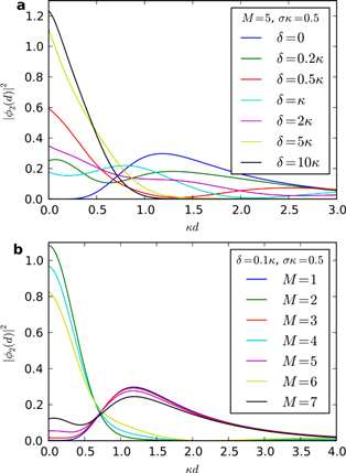
Figure 3. Two-photon scattering off M-atoms. (a) Scattering of the Gaussian two-photon wavepacket, equation (13), off M = 5 two-level emitters as a function of the relative coordinate  . The results change qualitatively from antibunching at small
  to bunching at large
  . (b) The same dependence as in (a) for fixed
  and various numbers of emitters M. The result exhibits the clearly pronounced parity effect of equations (23), (24).
Download figure:
Standard image High-resolution imageA much richer structure of an outgoing wavefunction appears at a finite detuning  . Assuming now
  , we observe that it develops a polynomial dependence on d

where the polynomial of the order 
has complex-valued coefficients.
At a large detuning  the elastic scattering dominates,
  turns into the Laguerre polynomial
  with the real-valued coefficients, and
  exhibits the same behavior as the one-photon scattering function (8): the probability
  oscillates on the scale κ−1 featuring precisely
  nodes. We note that the real-valuedness of the coefficients of
  is important for the presence of the nodes in
  , which are destroyed at a small detuning
  by the emerging effective interaction between photons.
Thus, tuning  from
from  to
to  we observe a qualitative change in the scattering properties (see figure 3(a)), characterized by the increasing role of the inelastic processes. The formation of bound states, transitions from bunching to antibunching, and the clearly pronounced parity effect give full evidence of strong correlations between photons resulting from their scattering off arrays of emitters in a 1D chiral channel.
2.3. Robustness of correlated states
It has been already discussed above that scattering results are independent of the positions of emitters, which ensures their robustness against fluctuations of the latter. Next, we study how robust scattering results are with respect to randomness in the emitters' transition frequencies. To this end, we consider detunings  as random variables which are normally distributed around the mean value
  with the variance Σ, and evaluate the probability distribution
with the help of the exact expression for  based on equation (12). In figure 4 we plot typical results of this averaging showing mean values as well as median and mean absolute deviations of the distribution (30). We observe that for not so large
  , this distribution is sufficiently narrow so that it does not mask the qualitative effects (parity, antibunching, etc) discussed above. Thus, we conclude that our results are robust with respect to the fluctuations in transition frequencies as well.

Figure 4. Two-photon scattering off M-emitters with random transition frequencies. (a) The scattering of a Gaussian two-photon wavepacket off M = 3 two-level emitters averaged over the fluctuating transition frequencies. The latter are modeled by independent random variables which are normally distributed around the mean value  with the variance Σ. The solid lines correspond to the mean values of the distribution (30). The filled regions denote the median (darker) and mean (lighter) absolute deviation. (b) The same dependence as in (b), but for M = 4 emitters. Both figures demonstrate that the qualitative properties of scattering states are robust against the fluctuations in the transition frequencies.
Download figure:
Standard image High-resolution image2.4. Effect of losses
To estimate an effect of losses due to the spontaneous emission out of the 1D modes we can again use the formulas (16)–(18), replacing  , where
  is the spontaneous emission rate (considered to be small
  ). After this replacement the scattering matrix is no longer unitary, which means that the norm of photonic wavefunctions is not preserved. To what extent does this modify the parity effect? By an explicit calculation for
  one can find that
 and
and 
 . The terms
  in the latter expression estimate (when divided by κ): (a) which part the norm of an initial two-photon wavepacket leaks out of the 1D channel; (b) a deviation from the full restoration of the initial wavepacket shape after scattering off two emitters. On this basis we conclude that the deviation
  from the perfect parity effect is accumulated on each scatterer, and thereby it is proportional to
  .
.
3. Discussion
We have suggested a novel approach to producing strongly correlated states of two and more photons in a highly controllable way. Our setup uses the edge states of photonic topological insulators with multi-level emitters coupled to it. The scattering in this setup possesses the following universal features.
First, multi-particle scattering does not depend on the positions of emitters. This is a general consequence of the absence of backscattering, and it makes the scattering outcomes robust against the fluctuations in the emitters' coordinates. This property also provides us with a powerful theoretical tool for calculating the scattering results based on the convolution property (4).
Second, the scattered wavepacket has a polynomial structure and the minima of the outgoing pulse are given by the zeroes of this polynomial. In particular, single-particle scattering (and the reducible part of multi-particle scattering in general) is described by Laguerre polynomials. In single-photon scattering, the outcome looks like a wavepacket fragmented between the nodes—the zeroes of this polynomial. The emergence of the nodes is accounted by time delays on each emitter. This leads to the non-monotonic behavior of the G2 correlation function thus signifying correlation between photons. In multi-photon scattering, this picture takes place at large detunings  , i.e., in the regime where the elastic processes dominate over the inelastic ones.
Third, the role of the inelastic processes enhances as we tune to small values of  . These processes lead to the emergence of the effective interaction between photons, which lies at the origin of the exciting effects: the parity-dependent scattering and the antibunching of photons. In particular, we have observed for the first time that at a vanishing detuning the two-photon scattering matrix in the chiral edge channel only depends on the parity of the number of emitters, and does not depend on the number itself. We substantiated our observation by the fundamental symmetry arguments. For an even number of emitters, we proposed certain array configurations which are transparent to arbitrary two-photon wavepackets. For an odd number of emitters, we discussed how to adjust the parameters of the initial two-phonon wavepackets in order to observe the antibunching behavior—the effective repulsion of photons—in the 1D geometry.
The physical picture behind the parity effect is the following. After the first incident photon is absorbed by the first emitter, the latter becomes transparent for the second photon. Thus, the first photon is delayed by the time  with respect to the second photon. This leads to antibunching of photons via scattering on a single emitter. If the second emitter is present, it absorbs the second photon and captures it during the time
  . This gives the first photon a possibility to compensate the lag, and both photons end up with the same relative distance as it was in the incoming state (note that the compensation is exact, only if the resonance condition is fulfilled, and if the emitters are identical). Repeating these arguments for odd and even numbers of identical emitters, we observe that the net result is the same as for one and two emitters, respectively. Deviations from the perfect conditions would lead to a difference between scattering results on, say, M = 1 and M = 3 emitters, but they still remain closer and qualitatively similar to each other, than to a scattering result on M = 2 emitters.
These exciting effects result from the combination of the reduced dimensionality, which increases the role of the photonic correlations, and the topological origin of the chiral edge states propagating without the backscattering. For their experimental observation, we specify below the necessary physical parameters. Photonic correlations are a vital ingredient for building up working schemes of future photonic quantum technology [5]. We believe that the effects described here will be used in future functional quantum photonic devices or for quantum simulation of condensed matter systems using photonic setups.
Physical realization. To observe the quantum many-body effects of photons described above one needs a photonic topological insulator analogous to the one studied in [34, 35]. The role of emitters can be played by either quantum dots or superconducting qubits, like, e.g., in [11] and [17]. Available single-photon emitters made of quantum dots and coupled to photonic crystal waveguides [9, 12, 20] can also serve for a realization of our model. Typical bandgap frequencies of existing photonic topological insulators lying in the GHz range match with the transition frequencies of single-photon emitters, which are necessary to inject photons into the 1D channel. The parameters provided in [34] allow us to estimate the topological photonic band gap  0.27 GHz as well as the group velocity
  . The electromagnetic field is bounded within an area of
  1600 mm2, which gives
  . The dielectric host material has a relatively large dielectric constant (see the Method summary section of [34]). On the basis of (1) we conclude that the Purcell factor of the setup of [34] is of the order of a few tens. The other setup described in [39] is made of an array of helix-like waveguides with the radius R. The spectral gap and the group velocity of the edge state (see figure 2(c) of [39]) depend nonmonotonically on R; the group velocity can even go down close to zero at
  m, rendering
  very large. This leads us to much more optimistic values of
  and a Purcell factor of the same order. A similar analysis of the third setup presented in [38] yields a Purcell factor
  20. A further enhancement of the Purcell factor in the near future can facilitate the experimental realization of our proposal.
In this paper we discussed the scattering results in arrays of two-level emitters. The present consideration, however, can be generalized to arrays of three- and four-level emitters, which are interesting due to the experimentally observed effects [8, 56, 57] of the single-emitter electromagnetically induced transparency and the transistor-like behavior, and the recent proposals to implement four-level emitters in the engineering of quantum gates, e.g. CNOT [58]. By combining emitters of different level structures one gains flexibility and the ability to build optical schemes with desired correlations of the outgoing photonic wavefunctions. For an explicit evaluation of the outgoing state one can use the scattering formalism of [47] in combination with the convolution property (4).
Currently available topological photonic crystals operate in the GHz frequency range. This is related to the difficulties in creating a large magneto-optical response with existing materials, which is needed for a nontrivial topology of the band structure. However, some recent developments [59] in material science might lead to a significant enhancement of the magneto-optical response in the optical domain, which can be used to engineer topological photonic crystals in the optical range of frequencies.
Finally, we note that interacting photons in two dimensions can lead to anyonic statistics and fractional Hall states [60]. The recent suggestion of realizing Dirac cone structure [62] may pave the way to exotic physics of interacting two-dimensional photonic fluids. Moreover, the recent classification of interacting bosonic topological insulators [61] suggests a possible route to engineer other exotic states of light.
We expect that the novel correlated states of photons and other propagating bosons will find applications in quantum information technology, optomechanics, and precision measurements.
Acknowledgments
We would like to thank D Baeriswyl, D Fioretto, and V Yudson for useful discussions. MR and VG are supported by MaNEP and Swiss NSF. MP is supported by DFG-FG 723 and 912. VG thanks KITP for hospitality.
: Appendix: Technical details
In the case of two-level emitters and identical couplings the model (2) is exactly solvable by the Bethe ansatz [53]. For a more general problem involving arrays of emitters with an arbitrary level structure, a complementary diagrammatic approach to scattering is available [47].
Below we provide the derivation of formulas appearing in the main text based on these approaches.
Appendix. Single-photon scattering
First, we rewrite the single-photon scattering matrix (6) in the coordinate representation
The corresponding scattered part  is given by
In the limit  ,
,  we obtain

where  are the associated Laguerre polynomials and CmM are the binomial coefficients.
Appendix. Two-photon scattering
The two-photon scattering matrix (12) can be parameterized by the detuning  (recall that the total energy
  is conserved) and the two relative coordinates
  and
and  .
.
First, we separate elastic and inelastic contributions to (12). Picking the unity in the square brackets in (12), we see that the two integrations disentangle, and we recognize the elastic contribution  to the two-photon scattering matrix (10). The remaining term in the square brackets in (12) generates the inelastic contribution
where

The elastic (reducible) part can be cast to
Evaluating this integral in terms of the Mth order residues, we obtain the contributions (16) and (17).
The inelastic (irreducible) part (A.5) admits the integral representation
which helps to decouple the sums over indices a and b. Assuming in the following  and employing the identities (see equation (A.4))
we transform (A.8) into
Integrating over τ we obtain
The second term exactly compensates the contribution from the pole  in the first term. So we can rewrite (A.13) as
where the contours of integration are deformed to the small circles  and
and  embracing clockwise the poles
  and
and  , respectively.
Transforming (A.13) plus its complements  to the mixed representation of the total energy
  and the relative coordinates
  , we obtain
where  , and the contours
  and
and  embraces the origin clockwise. Noting that
we cast (A.15) to
Representing

where  is a polynomial of the degree
  , we establish the identity

and hence
With its help we further transform (A.17) and obtain the contribution (18).
At  equation (18) amounts to
Footnotes
- 5
It should be remembered that
 only for , since in the region the scattered part is masked by the non-scattered part .


