


Abstract
We present a method to utilize interatomic Coulombic decay (ICD) to retrieve information about the mean geometric structures of heteronuclear clusters. It is based on observation and modelling of competing ICD channels, which involve the same initial vacancy, but energetically different final states with vacancies in different components of the cluster. Using binary rare gas clusters of Ne and Ar as an example, we measure the relative intensity of ICD into (Ne+)2 and Ne+Ar+ final states with spectroscopically well separated ICD peaks. We compare in detail the experimental ratios of the Ne–Ne and Ne–Ar ICD contributions and their positions and widths to values calculated for a diverse set of possible structures. We conclude that NeAr clusters exhibit a core–shell structure with an argon core surrounded by complete neon shells and, possibly, further an incomplete shell of neon atoms for the experimental conditions investigated. Our analysis allows one to differentiate between clusters of similar size and stochiometric Ar content, but different internal structure. We find evidence for ICD of Ne 2s−1, producing Ar+ vacancies in the second coordination shell of the initial site.
Export citation and abstract BibTeX RIS

Content from this work may be used under the terms of the Creative Commons Attribution 3.0 licence. Any further distribution of this work must maintain attribution to the author(s) and the title of the work, journal citation and DOI.
1. Introduction
The determination of cluster structure and size is a problem yet unsolved. In particular, this is true for heterogeneous (or binary) clusters. Here we introduce a new method to obtain detailed information on the size, composition and structure of clusters. This method is applied to the system of mixed neon argon clusters formed by coexpansion of the two gases. We used five different expansion conditions to produce mixed cluster ensembles of different mean size, composition and structure. We then obtained the most likely structure for each ensemble by comparing our experimental spectroscopic data to simulations. Our method utilizes the experimental analysis and theoretical simulation of interatomic Coulombic decay (ICD) involving either Ne–Ne or Ne–Ar atom pairs in the clusters produced. As the range of the dipole–dipole interaction mediating ICD is short, both the energy of ICD electrons as well as the ICD decay width are crucially dependent on the type, number and position of the nearest neighbors of the decaying atom.
In the ICD process the initial vacancy on, e.g., atom A is filled by an electron of the outer valence shell of the same atom. Instantaneously the excess energy is transferred via a virtual photon to a neighboring atom B, which is ionized in the course of the transition and produces the ICD electron being emitted into the continuum. Afterwards the two resulting positively charged atoms repel each other and undergo Coulomb explosion. This mechanism was theoretically predicted by Cederbaum et al [1] and later verified experimentally in neon clusters [2]. Since then several other ICD-like processes have been proposed and have been further investigated on numerous weakly bound systems, such as noble gas clusters of different sizes, hydrogen-bonded systems or substrates attached to enzymes [3]. The experimental status and the theory of ICD have been reviewed in [4, 5]. Of particular interest for this work is the experimental evidence of a very efficient ICD in neon clusters [6, 7].
Theoretically, the decay widths of ICD and ICD-like processes have been investigated for very small clusters of 2–13 atoms using several approaches, such as Wigner–Weisskopf-theory [8], CAP-CI [9] and FanoADC–Stieltjes [10]. The latter scheme was established to be the best compromise between computational cost and accuracy. Further studies of model structures of ArXe clusters have been carried out using the asymptotic approximation [11]. In this approach to the ICD electron spectra of heteronuclear ArXe clusters, a linear combination of fcc and hcp model structures [11] was investigated leading to the observation that the peak positions as well as their intensities sensitively reacted to slight changes of the chosen geometries.
In this work, the ICD spectra for NeAr clusters were experimentally reinvestigated. These mixed clusters are of special interest because both Ne–Ne pairs as well as Ne–Ar pairs can undergo ICD after ionization of the Ne 2s shell. Decays into  and
and  final states are therefore competing processes. In these new measurements not only was the NeAr ICD measured as in [12], but also the NeNe ICD, which is now properly resolved due to technical improvements (this paper). In experiments on the neon dimer, the NeNe ICD lifetime was found as
  [13], while the NeAr dimer ICD lifetime was calculated to be 36 fs [14]. From this one would conclude that the NeAr ICD peak dominates the ICD electron spectrum. As we will show below, this assumption is not generally correct for the structured, hetero-nuclear clusters investigated in this work.
Both small neon clusters as well as the NeAr dimer have previously been studied in detail. For pure neon clusters the decay width has been found to scale faster than linearly with the total number of atoms, until the first solvation shell around a central atom is closed at Ne13 [8, 15]. This is easily explained by the influence of the neighboring atoms on the ionization energies within the clusters. Inner valence holes are less stabilized than outer valence holes. Hence the energy difference is decreased with increasing cluster size. The decay width of one pair in the asymptotic approximation is proportional to  [11], where ωvp denotes the energy of the virtual photon. Therefore the decay width scales not only with the number of atoms but is additionally enhanced by the stabilization of the ionized states. However, this effect is very local and for clusters with two or more shells of atoms around the ionized site, it will be approximately constant.
The relative intensities of the NeNe ICD and the NeAr ICD peaks as well as their shapes strongly depend on the expansion conditions. We interpret those as different mean structures and will compare the experimental results to theoretically modeled spectra using several idealized geometries as an approximation to the true cluster structures. By this we take a first step in utilizing ICD as a tool for structure analysis.
Several other experimental techniques and theoretical methods have been used to investigate the structure, size and composition of clusters. For homogeneous systems, experiments using mass spectroscopy [16–19] were followed by particle scattering of a He beam [20]. Analysis of photoelectron spectra allowed one to disentangle contributions of different cluster sites in some cases [21]. Most recently, scattering of intense x-ray beams [22] and other spectroscopic techniques [23, 24] (to name just a few) considerably enhanced the insight into this subject.
Results for heterogeneous clusters are less detailed. For mixed rare gas systems, fluorescence spectroscopy allowed for insights into the geometric and electronic structure [25–27], and photoelectron spectroscopy probed other aspects of these systems [12, 28–30]. Thermodynamical considerations [31, 32] and molecular dynamics (MD) simulations [33, 34] have been an important line of research for theory.
In this investigation we combine a theoretical model with experimental results to obtain a wide range of structural information on mixed clusters which exhibit two discernible ICD features in their electron spectra. We can obtain the cluster size, structure and composition of the cluster ensemble simultaneously. This could not be done with such accuracy before. In our approach we need two distinguishable ICD features in the electron spectrum, however, the method is not limited to this feature. Instead, any two competing ICD-like processes with comparable lifetimes that carry information about the surroundings and are spectroscopically resolved could serve as a basis for structure determination. If it is known with certainty that only two processes can occur, the measurement of one secondary electron would be sufficient for the characterization of both competing processes.
The paper is structured as follows: in the next section we briefly summarize the experimental details, describe the measured spectra and summarize all relevant experimental parameters. The theoretical methodology is explained in detail in section three. In section four we provide the motivation for and introduce the cluster structures we considered. For these structures we calculated the expected NeAr and NeNe ICD contributions. In section five we discuss the theoretical findings, compare them with the experimental results and draw conclusions on the actual cluster structure and size of the five different cluster sets. Section six concludes this work. An incomplete set of the agreement plots between experimental and theoretical calculations for all calculated structures can be found in the appendix.
2. Experimental details
2.1. Experimental methods
The experiments described here were performed in single-bunch operation at the dipole beamline TGM 7 of the synchrotron radiation facility BESSY II at Helmholtz-Zentrum Berlin. All spectra were recorded using slit widths of 300 μm. The resulting bandwidth of the synchrotron radiation was approximately 60 meV for the measurement of the outer valence spectra at 22.43 eV and 150 meV for the measurement of the coincidence spectra at 52.1 eV. Clusters were produced by expansion of a mixture of neon and argon through a cryogenically cooled, conical copper nozzle [35]. The nozzle had a diameter of 80 μm and an opening angle of 15°. In order to produce clusters of different size and composition we varied the initial mixing ratio of Ne and Ar in the expanding gas, the temperature of the nozzle and the expansion pressure. Table 1 summarizes these parameters. Note that the values given for the mean cluster sizes  and
and  were calculated using a formalism made for homogeneous clusters [36]. The values given can therefore only be an estimate for the general dimension of the size of the final clusters.
Table 1. The expansion parameters of NeAr gas mixtures used to produce different cluster ensembles. In the fourth (fifth) column, we give the cluster sizes that would result for an expansion of pure Ne (Ar) gas at the given nozzle size, temperature and stagnation pressure, according to an empirical formula by Hagena [36].
| Designation | Ar content in | Expansion | Nozzle |

|

|
|---|---|---|---|---|---|
| initial mixture | pressure | temperature | |||
| Set 1 | 1.7% | 0.26 bar | 63 K | 5 | 520 |
| Set 2 | 7.4% | 0.40 bar | 60 K | 17 | 1850 |
| Set 3 | 1.7% | 0.25 bar | 57 K | 7 | 810 |
| Set 4 | 7.4% | 0.24 bar | 58 K | 6 | 670 |
| Set 5 | 1.0% | 0.16 bar | 54 K | 3 | 380 |
For electron detection, we used a magnetic bottle time-of-flight spectrometer. Details of this instrument and its operation are described in [37]. Conversion of time-of-flight data to kinetic energies was performed as described in [38]. The stability of expansion conditions was monitored by measuring outer valence spectra before and after each measurement of the ICD spectra. The valence spectra also allowed as to estimate the relative content of neon and argon in the final clusters, which is very different from that in the initial mixture. Details of this are described in the next section. ICD spectra were taken at an excitation energy of 52.1 eV. Thus, the Ne 2s photoline lies in between the kinetic energies of the Ne–Ne and the Ne–Ar ICD and hence allows for optimal energy resolution. To determine the contribution of Ne–Ar and Ne–Ne ICD to the respective coincidence spectrum, the area of the Ne–Ar and Ne–Ne ICD peaks was measured by integrating the respective features after a background was subtracted.
2.2. Experimental results and discussion
The outer valence spectra of the cluster ensembles are shown in figure 1. In addition to the contribution of the cluster bands, spectroscopically distinct features of uncondensed monomers, which are also present in the gas jet, are seen for Ne. The Ne 2p monomer peak is by far the most intense contribution in all measured spectra and is not shown to full height. The Ar 3p monomer contribution to the total spectrum is small compared to the Ar 3p cluster contribution, and its presence is not clearly resolved from the structure of the cluster valence band [39, 40]. The double structure visible in the Ar peak for most cluster sets is interpreted as the maximum of the cluster valence band (low binding energy peak) and the unresolved Ar 3p and 3p
 monomer contribution (high binding energy peak). This interpretation is corroborated by additional spectra of the Ar peak structure at higher energy resolution (not shown). It is thus seen that most of the argon is condensed, while most of the neon atoms are uncondensed. This is expected, because under the chosen expansion conditions, neon would only form very small clusters (compare table 1) while the condensation of argon might even be enhanced if the co-expanding neon functions as a seeding gas. As the freezing point of Ar is much higher than that of Ne, few Ar atoms were expanded together with a much higher fraction of Ne atoms, and at temperatures which are too high for the formation of pure Ne clusters. At lower temperatures, or higher fraction of Ar atoms, stable operation of the gas jet is not warranted because of Ar freezing inside the nozzle.

Figure 1. Outer valence spectra of coexpanded NeAr gas mixtures, recorded at a photon energy of 22.4 eV. The Ne 2p and Ar 3p outer valence bands are shown. The labelling of the traces refers to the expansion parameters as delineated in table 1 and hence to different mixtures of clusters with different mean cluster sizes. This color coding is going to be used throughout the paper. For Neon, besides the cluster contribution a strong monomer line can be seen at a binding energy of 21.6 eV.
Download figure:
Standard image High-resolution imageThe width of the outer valence spectra can be used as an indicator for the relative cluster size within the different sets. As a measure for that we used the energy position of the low energy flank at half the maximum peak height to compare the relative widths of the bands. In detail, we used the lower binding energy at half the peak height of the respective cluster band. The amount of Ar present in the clusters was calculated from the areas of the outer valence cluster bands, with the approximate contribution of monomers subtracted after a peak fit. This procedure is the main source of experimental error in the Ar content of clusters (see below). These values were then corrected using the respective atomic photoionization cross sections at an excitation energy of 22.4 eV as given in [41]. The use of atomic cross sections for van der Waals clusters seems justified from the weak bonding, and has been underpinned by experiments at least for Ar [39].
When the photon energy is increased above the Ne 2s ionization threshold (around 48.5 eV in Ne atoms, and 48.1 eV in larger Ne clusters [4]) low kinetic energy electrons due to ICD start to appear. In figure 2, we show the energy spectrum of the ICD electrons at a photo excitation energy of 52.1 eV, filtered to display only events in which an electron has been recorded in coincidence with a photoelectron from the Ne 2s cluster band. At the given excitation energy this band lies in the kinetic energy region of 3.8–4.8 eV. The corresponding region of the ICD electron is not displayed in figure 2, because two electrons cannot be measured simultaneously. This is due to the dead time of the constant fraction discriminator of approximately 25 ns after any electron hit [37].
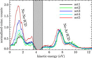
Figure 2. The Ne–Ne and Ne–Ar ICD spectra of coexpanded NeAr gas mixtures. The energy distribution of all electrons which are detected in coincidence with an electron in the Ne 2s binding energy region is shown. The spectra have been normalized to the maximum of the Ne–Ar ICD peak. Secondary electrons with an energy identical to the primary Ne 2s photoline cannot be detected in our set-up. The respective energy region is hatched in the figure. Labelling of the traces is the same as in figure 1.
Download figure:
Standard image High-resolution imageThe coincidence spectra mainly consist of two distinct features. Electrons resulting from ICD of a Ne 2s vacancy into a (Ne+ 2p−1)2 final state ('Ne–Ne ICD') are seen at a kinetic energy of approximately 1.5 eV. This feature is approximately 1.5 eV wide. Any possible substructures within this feature cannot be identified with certainty. It is not expected that the calculated substructures of this peak (compare with figure 6) can be observed easily in the experiment because the calculations are based on one single cluster while the measurements were made on an ensemble. The second distinct feature, pertaining to ICD into a (Ne+ 2p−1 Ar+ 3p−1) final state ('Ne–Ar ICD') is observed in the kinetic energy range of approximately 6.5–10.5 eV. It is a double peak structure where the main peak has its maximum at approximately 7.7 eV and the smaller peak has a maximum at approximately 9.2 eV. In order to obtain a measure of the Ne–Ar ICD contribution to the total ICD contribution we measured the area under the respective ICD features after a linear background was subtracted.

Figure 6. Calculated ICD electron spectra for the structures showing the best agreement to the experimental argon content and NeAr ICD to total ICD ratio (table 4). The intensities are normalized to the peak height of the NeAr ICD peak and the spectra are convoluted by Gaussians with a width of 250 meV. The simulated spectra nicely match the experimental ones in figure 2. Both, the NeNe ICD peak at low energies and the NeAr ICD peak at higher kinetic energies show a peak structure which results from differences in the distances of the atom pairs involved in the process. See the text for details.
Download figure:
Standard image High-resolution imageResults from the analysis of the spectra in figure 2 are collected in table 2. Uncertainties given for the Ar content take into account the statistical error of the area and a 10% uncertainty in the respective outer valence cross sections, which allows for a—yet hypothetical—deviation of the outer valence photoionization cross sections for clusters from those of the respective atomic orbitals.
Table 2. Experimental results. The cluster band onsets are given at half the peak maximum of the respective feature. The percentage of Ne–Ar ICD is referred to the summed area of both ICD lines.
| Designation | Ar content in | Onset Ar 3p | Onset Ne 2p | Ne–Ar ICD |
|---|---|---|---|---|
| final cluster | cluster band | cluster band | contribution | |
| Set 1 | 47 ± 10% |
 eV eV |
 eV eV |
63 ± 7% |
| Set 2 | 35 ± 5% |
 eV eV |
 eV eV |
61 ± 10% |
| Set 3 | 21 ± 4% |
 eV eV |
 eV eV |
38 ± 5% |
| Set 4 | 20 ± 4% |
 eV eV |
 eV eV |
53 ± 6% |
| Set 5 | 8 ± 2% |
 eV eV |
 eV eV |
28 ± 3% |
The results, and in particular their implications on the interpretation of the cluster structures, will be discussed below (section 5). In brief we can say that a wide range of different cluster ensembles was produced. We can further assume that the produced clusters are mixed. Otherwise, we would not see a contribution from Ne–Ar ICD.
3. Methods
A secondary electron spectrum as shown in figure 2 is characterized by the kinetic energy of the emitted electron and the corresponding intensities. In the following we delineate our approach to simulate such spectra theoretically. As shown in [11] we write the energy of the ICD electron as

where SIP denotes the single ionization potentials of the initially ionized atom A and the electron-emitting atom B. R denotes the internuclear distance of the atoms, and Ein the ionization potential of the inner valence level that decays via ICD. The latter is assumed to be a constant, which is an approximation that holds for weakly bound systems with flat potential curves. Otherwise the initial state energy has to be treated more accurately [5].
NeAr dimers can accomodate four vibrational levels in the electronic ground state. The population of these levels influences the kinetic energy of the ICD electrons as well as the decay width but for the current investigation we assume the clusters to be in the vibrational ground state. Additional aspects to be addressed later are the transferability of the dimer results to clusters with a more complex potential, and a possible steric hindrance of vibrations by neighboring atoms.
The estimation of the corresponding intensities needs a more sophisticated approach. From a theoretical point of view the intensities of the peaks in a secondary electron spectrum can be understood as transition probabilities from some initial state into certain final states, which will later be defined according to the physical problem. They are hence proportional to the decay rate and as such to the decay width Γ. The decay width is accessible via Fanoʼs golden rule [42] for autoionization processes:

where H is the Hamiltonian of the full system, Φ denotes a bound state describing the initial state leading to a resonance energy  , and
, and  is a specific final state β of energy ε with appropriate boundary conditions. The initial and final states are coupled through the Coulomb interaction between the electrons of the systems.
The eigenfunctions  form a complete set of basis functions. Therefore the above equation (2) can be expressed within another complete basis of continuum functions. As true continuum wavefunctions are difficult to use from a numerical viewpoint, schemes to approximate this basis by a discrete set of
  basis functions have been created. The utilization of excited two-hole-one-particle (
 ) functions obtained in the algebraic diagrammatic construction (ADC) scheme [43], is one possible choice. This ansatz is called FanoADC [10] and hence the decay width is obtained as
where q denotes those  configurations that were selected for the description of the final states. Subsequently, the discrete spectrum needs to be smoothed and renormalized, which we do by employing the Stieltjes method [44].
The distance dependence of the NeAr dimer decay width was calculated non-relativistically for a number of points covering the distances that occur in the cluster. We have used the Fano–Stieltjes procedure implemented in DIRAC [45, 46] with an aug-cc-pV6Z basis set on both atoms. Five additional basis functions each of s, p and d orbitals of the KBJ type [47], were introduced residing at the geometric center of the dimer.
Since inversion symmetry is not yet accounted for in our program, we are going to use calculated decay width data from the literature for the Ne dimer obtained with the same method and a comparable basis set [48].
Quantitatively, we have used lifetimes of 60 fs for a Ne–Ne pair and of 44 fs for a Ne–Ar pair, at their respective equilibrium distances. The lifetime of  fs measured for the Ne dimer [13] deviates from the one given. So far the lifetime of NeAr dimers has not been measured experimentally. For the current investigation, however, it is most important to achieve a consistent description for both the NeAr and NeNe systems. We have therefore decided to use the theoretical values, calculated on an equal footing in both cases. The decay width can then be estimated by the sum over all possible final states for every atom pair in a given structure. In the summation, the exact distance dependence of the widths is found by interpolation between a number of reference points. We thus arrive at a computationally cheap method for the description of systems consisting of many atoms, such as clusters.
All calculations were performed using the HARDRoC [49] program, which evaluates the decay widths for a given input structure and given (experimental) ionization potentials. Values used in this article are listed in table 3. The figures for the Ne 2s and 2p ionization potentials correspond to the minimal binding energy at which the respective peak becomes visible. Using experimental ionization potentials, we avoid exactly calculating the stabilization of singly and doubly ionized final states due to polarization charges.
Table 3. Experimental values for the single ionization potentials (this work) used for the estimation of the decay widths.
| Indicator | Value |
|---|---|
| SIP(Ne2s) | 47.75 eV |
| SIP(Ne2p) | 21.10 eV |
SIP(Ar3p) |
15.40 eV |
SIP(Ar3p) |
15.20 eV |
We now consider the accuracy of our procedure. Errors can arise mainly in the Fano–Stieltjes procedure and by the choice of static structures in the ground state. In reality the atoms within the cluster are going to oscillate and the considered geometries only reflect an average configuration. Rigorous estimates for these uncertainties and their propagation are currently not available. However, we would like to point out a trend for an error cancelation mechanism that can be explained employing the example of a NeArNe trimer. For this system, a lot of the uncertainty results from the oscillation of the argon atom along the internuclear axis of the two fixed neon atoms. By that however, ICD of a vacancy on one of the Ne atoms gains in intensity, while the decay of the other Ne site loses intensity. For a linear distance dependence of the ICD rate it is obvious that these two trends will cancel exactly, and even for an  behavior of the decay width often assumed for ICD [10], cancelation occurs in this model system. We believe this effect prevails even in larger systems. The error of the NeAr ICD would then only depend on the accuracy of the FanoADC calculations. We only draw conclusions about the mean values of the NeAr ICD to total ICD ratio and hence the information is already available at this stage, while the explicit quality of the approach needs further investigation.
This ansatz of decomposing the cluster into a manifold of pairs, with all atoms of the same atom type having the same ionization potentials, does not take into account the dependence of the ionization potentials on the sites of the atoms within the clusters, but averages over these effects. We find that this approach gives a reasonable approximation for the desired quantities. Its advantage is the low numerical cost which allows its application especially to large systems otherwise not accessible.
4. Simulated structures of NeAr clusters
Small noble gas clusters preferably form icosahedral structures, while with increasing cluster size an fcc structure becomes more favorable. From energetical arguments alone, this transition would occur at cluster sizes in the range from 750 to 3500 atoms [31, 50, 51]. Experiments on pure Ar clusters produced by supersonic expansion give a somewhat less clear-cut picture, as signatures of both local motifes appear simultaneously for cluster ensembles starting at a mean size somewhere between 200 atoms [52] and 750 atoms [53, 54]. Evidence for a similar situation has been presented for Ne clusters with  [55]. For our simulations we assume that the clusters have icosahedral structure. For all sets except for set 2 the expansion conditions should result in clusters with mean sizes below 750 (see table 1). The mean size of the clusters of set 2 is well below 3500.
The actual cluster formation process is understood as follows. First, a three particle collision has to take place to form argon dimers. Subsequently, single atoms are added to the dimer due to collisions. At a later stage these clusters can also collide to form larger clusters. This process, called coagulation, becomes the dominant one for the formation of very large clusters.
Earlier results on NeAr mixed clusters have been obtained by luminescence spectroscopy [27, 56], MD simulations [33, 34] and photoelectron spectroscopy [12]. The latter work is based on the observation of energy positions and band widths. In it co-expanding NeAr mixtures were found to form core–shell systems with an Ar core covered by one or several Ne layers. This seems plausible also from a thermodynamical viewpoint [57]. The other works considered clusters formed by pick-up, which does not necessarily lead to the same structures. Nevertheless, for the case of large Ne clusters doped with few impurity Ar atoms, the Ar formed a compact assembly inside the host clusters [27, 56]. The MD simulations considered the reverse situation, namely pick-up of Ne by Ar clusters. Again, the Ne atoms did not diffuse into the Ar bulk, in contrast to other binary rare gas mixtures. Given this evidence we take core-shell systems as a starting point for our simulations of the average structure of the clusters in our study.
The icosahedral core of argon atoms used in all of our simulations is shown in figure 3. In this example, it has an edge length of  atoms and consists of
  , which can be calculated from [50]

For the construction of the structure we assume the minimum distance between two argon atoms to be twice the van der Waals radius of argon,  = 1.88 Å [58]. We have constructed further shells such that the distance
  is maintained between two surface atoms; consequently, the distance of two atoms in the edges is slightly increased [50].
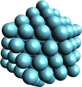
Figure 3. An icosahedral argon cluster with an edge consisting of  atoms, containing 147 atoms, distributed over four shells. 55 atoms belong to the core, 12 are at the vertices, 60 in the edges and 20 inside the surfaces.
Download figure:
Standard image High-resolution imageAs we are going to see in the discussion, the outcome of the experiment cannot be explained solely by assuming that an argon core is surrounded by complete neon shells. We will therefore consider other conceivable cluster structures which consist of an argon core surrounded by neon atoms in different ways. We use four different types of clusters, with examples shown in figure 4. In order to describe these clusters we use the following variables and nomenclature:
- (i)
 —edge length of argon core, i.e. number of layers,
 - (ii)—number of complete neon shells around the argon core,
- (iii)—number of covered triangular surfaces (out of 20) (compare with figure 4(b)),
- (iv)—number of covered triangular surfaces by filled caps (compare with figure 4(c)),
- (v)—randomly arranged neon atoms around the outermost complete shell to fulfill the Ne–Ar ratio criterion (argon content in %).


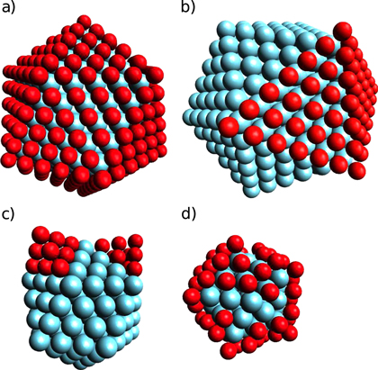
Figure 4. The four different structure classes considered in our calculations (see text for nomenclature). (a) Complete shells, here  ,
,  . (b) Incomplete shells, here
  ,
,  ,
,  . (c) Caps, here
  ,
,  , caps = 2. (d) Randomly arranged neon atoms around a full shell cluster, here
  ,
,  ,
,  .
.
Download figure:
Standard image High-resolution imageIn the case of an argon cluster surrounded by one or more complete shells of neon, first the core structure is created and afterwards the outer shells are constructed around it, such that the minimum distance between a neon atom in the surface and an argon atom in the shell beneath is the sum over the van der Waals radii, where  = 1.54 Å [58] (see figure 4(a)).
The argon content determined experimentally does not correspond to the one expected for an Ar icosahedral core with completely filled Ne outer layers for all ensembles. Maintaining the idea of shells, we consider the occurence of incomplete shells. The cluster structures are created analogously to the complete shells except that not all triangular surface areas of the argon core are covered by neon atoms (for an example see figure 4(b)).
Another plausible structural motif is caps covering surface areas, as shown in figure 4(c). These structural elements do not exhibit minimum energy for clusters, but they might explain a large number of neon–neon interactions compared to the number of neon–argon interactions as seen in the experiments. The neon–neon distances within the caps are calculated in the same manner as described before for the (in-)complete shells. A whole manifold of distinct cap localizations is possible in principle, but it was observed that these different cap locations did not change the NeAr/NeNe ICD ratio for a constant number of caps. Since we are unable to distinguish these structures, we will limit ourselves to the discussion of structures containing a different number of caps.
A fourth conceivable structure consists of neon atoms randomly arranged around a homonuclear or heteronuclear cluster with complete shells, as shown in figure 4(d). It is constructed as a cluster with complete shells and afterwards neon atoms are added at random positions within the next layer until the desired  ratio is reached.
All structures are idealized and highly symmetric, which reduces the computational cost.
Vibrations inside the clusters will change the atom distances and hence both the kinetic energy of the ICD electron and the decay widths. For NeAr, the ICD processes are faster than dynamical rearrangements caused by Coulombic attraction after the initial ionization, or by vibrations [14]. In the case of the neon dimer, the ICD lifetime is comparable to the rearrangement time and hence influences the ICD electron spectra [59]. However, in clusters larger than the dimer the ionized atom can interact with more than one neighbor, which leads to an increase in the number of available final states. Hence the decay width increases, to first approximation linearly with the number of nearest neighbors. At the same time, the larger number of neighbors stabilizes the position of the initially ionized atom in space, compared to the dimer. Therefore we will assume that the structures given above are good approximations for the decaying clusters.
5. Results and discussion
We start with an interpretation of some general trends in the experimental set of cluster parameters (table 2) and compare the simulated results to the experimental data afterwards.
5.1. Experimental cluster structures
Data for the different cluster ensembles are shown in table 2 and sorted by decreasing relative Ar content. The position of the low binding energy flank of the cluster 3p line is an indicator for the absolute size of the Ar core. The trends in this parameter are mirrored by the cluster sizes inferred from Hagenaʼs rules (table 1) for all sets of expansion conditions except the first one. Also, for sets 2–5 the increasing size of the Ar core also goes along with increasing Ar content in the clusters and, for all sets, increasing Ar content is accompanied by increased degree of Ar condensation. Set 1 seems to be particular in this respect, as from the comparison to set 3, which was measured with the same gas mixture, a smaller Ar content and smaller Ar cores for set 1 are expected, a fact that cannot be explained in detail at the moment. The maximum of the Ar peak is at higher energy than for the pure Ar clusters  investigated in [39], and the spectrum of the latter looks more flat-topped. Pure Ar clusters produced in another experiment [60], at very different conditions, show more similarities to the current results. Therefore, it cannot be said here to which extent the shape of the Ar outer valence band is influenced by the Ne admixture.
In contrast to the argon results, the onset of the Ne valence structure is at a constant binding energy within experimental accuracy. The shape of the cluster Ne 2p line matches the one assigned to interfacial Ne layers in earlier work [29] and is clearly different from the one seen for pure Ne clusters. Thus, the experimental photoelectron data fit the picture of core-shell systems with Ar cores of different sizes, covered by one or few Ne layers. The mean argon core of set 5 is the smallest of all measured ensembles. Since the nearest neighbors account for most of the final state polarization, which leads to the observed Ar binding energy shifts, we assign these clusters to a core with either one or two filled shells ( or
or  ). (In other words, the core contains a single Ar atom, or an icosahedron consisting of a central atom and the first solvation shell.)
We now look at the ICD rates. For a Ne dimer at a distance of  , the calculated ICD rate is slightly smaller, but in the same order of magnitude, than for a NeAr dimer at
  . We can thus interpret the relative contribution of NeAr ICD as the fraction of nearest Ar neighbors of a Ne atom, averaged over all Ne sites in the cluster. Due to surface effects this number can easily exceed the average Ar content, e.g. for a Ne–Ar–Ne trimer, the Ar content is 33%, but the fraction of Ar nearest neighbors is at unity. It is thus plausible that the figure for the NeAr ICD contribution always is above the Ar content. We would like to point out though that it differs strongly between sets 3 and 4, which have otherwise identical parameters. Apparently, these ensembles are structurally different despite showing the same stoichiometry. Set 5, remarkably, still shows 30% Ne–Ar ICD at an Ar content below 10%.
5.2. Comparison to simulations
Our simulations yielded the ICD spectra for a large number of model cluster structures. In order to compare these with the experiment, a suitable metric is needed. We have chosen to use, for all clusters, the Ar content and the NeAr ICD intensity, both on a relative scale, for this purpose. In figure 5, as an example, we show simulated results for clusters consisting of an argon core with an edge size of  , surrounded by one complete shell of neon atoms
  , and a further, incomplete Ne shell, the filling of which is varied from
  (a single face covered) to
  (all except one face covered). These data points vary monotonically along the horizontal axis from right to left, as the relative Ar content decreases with increasing SNe. Each step further to the left corresponds to one more face of the cluster covered by a second Ne layer.
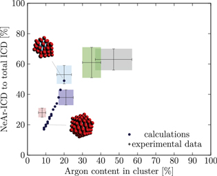
Figure 5. NeAr ICD to total ICD ratio plotted versus the argon content in the cluster. Experimental results are shown by error intervals and colored areas, at positions corresponding to the values given in table 2. Simulated results are shown by dots, and structures corresponding to  and
and  , respectively, are highlighted by pictures. The data for some values of SNe overlap. Ar content was rounded to integer values of the percentage. See the text for a full explanation of the theoretical data points.
Download figure:
Standard image High-resolution imageSimilar plots have been made for all simulated structures, and a selection of them shown in the appendix in figures A1–A24. Throughout the paper, including the supplementary material, we apply the same color coding to the experimental spectra as in figure 2, for which the relevant parameters are listed in table 2.
We deduce the most likely structures of the clusters on the basis of the agreement of the simulated values, plotted as in figure 5, to the experimental ones. Quantitatively, we minimize the following measure for the experiment-theory deviation:

where  and
and  denote the deviation of the argon content and of the relative NeAr ICD decay width, respectively. With the exception of set 5, only structures are considered, for which the argon content of the model structure lies within the error interval of the experimental data. For example, in figure 5,
  is an eligible structure for the clusters in set 4, and both
  and
and  are eligible for set 3. The simulated structures which minimize d are given in table 4.
Table 4. Structure parameters of the clusters giving the best fit to the epxerimental data. d is the graphical distance of the theoretical value to the experimental result, as in equation 5 and N denotes the total number of atoms in the cluster structure. Values set in italic are also plotted in figure 5. For set 4, only the random arrangement is listed for which the argon content matches the experiment.
| Set | CAr | CNe | SNe |

|
N | d |
|---|---|---|---|---|---|---|
| 1 | 4 | 1 | 1 | — | 330 | 2.000 |
| 1 | 5 | 1 | 2 | — | 610 | 4.472 |
| 1 | 2 | 0 | 5 | — | 29 | 4.472 |
| 2 | 3 | 1 | 0 | 35 | 157 | 1.000 |
| 2 | 3 | 1 | 1 | — | 162 | 3.162 |
| 2 | 2 | 0 | 8 | — | 36 | 4.123 |
| 3 | 2 | 1 | 3 | — | 77 | 4.000 |
| 3 | 3 | 1 | 7 | — | 218 | 4.123 |
| 3 | 3 | 1 | 8 | — | 224 | 4.472 |
| 4 | 2 | 1 | 0 | 20 | 65 | 2.000 |
| 4 | 2 | 1 | 1 | — | 65 | 4.000 |
| 5 | 2 | 1 | 13 | — | 125 | 8.246 |
| 5 | 2 | 1 | 14 | — | 131 | 9.220 |
| 5 | 2 | 1 | 15 | — | 134 | 9.220 |
We will discuss the structure assignment in descending order of the set number, which corresponds fairly well to increasing cluster size.
We start with set 5 (red). As mentioned above clusters in this ensemble are the smallest measured. These expectations are in agreement with the results of figure 5 (also to be found in the appendix in figure A9), where the red square can be matched with parameters of  ,
,  and another, almost complete outer neon shell with SNe between 13 and 20. None of the model clusters matches the experimental parameter range for the Ar content within the error bars, though. This might be explicable by assuming even smaller clusters, which do not have an icosahedral argon core, but only a coagulation of 2–11 Ar atoms plus a Ne outer layer.
Set 4 (turquoise) shows a very good agreement for a structure with  ,
,  and some additional atoms (see figures 5, A9 and A21). Whether these atoms are randomly arranged around the complete shells or are forming a contiguous set cannot be decided with certainty. From the geometric distance, the random arrangement is preferred.
The results for set 3 (blue) show a good agreement with structures of  or
or  ,
,  and
and  or
or  , respectively, as shown in figures A9 and A10. Structures containing randomly distributed Ne atoms in the outermost layers, instead of contingent sets covering some surfaces of the icosahedron, are in worse agreement with the experiment. In other words, for the clusters in set 3 a more contingent arrangement of Ne atoms leads to a propensity towards decay into
  final states, in comparison to set 4. We are thus able to distinguish the structures of two cluster ensembles with the same argon content by interpretation of the ICD spectra.
Set 2 (green) is assigned to a core size of  with one Ne outer layer
  plus some further neon atoms (see figures A5 and A10). Structures fitting best to the experiment have either
  or
or  , with the random arrangement slightly preferred. If we assume smaller clusters in set 2
  , the best fit is given by
  and
and  . This means that the argon core is surrounded by only half a shell of neon atoms. Some structures with larger core sizes (
 , corresponding to 309 core atoms) are almost within the experimental error range as well. Considering that both from Hagenaʼs approach and from the single ionization potential of the Ar 3p band, set 2 is supposed to have the largest Ar core, the latter structures might be closer to reality than the smaller ones with
  .
.
Due to the large error bars, the parameters of set 1 (black) are in agreement with a number of simulated structures. While the best fit is given for rather large Ar cores ( ) with a single layer of outer Ne and some further, contingent Ne atoms, also smaller Ar cores with incomplete Ne coverage (e.g.
  ), larger Ar cores (
 ) and clusters with
  and decorated with caps (figure A18) are within the experimental range of parameters. Since caps are energetically less favorable than the other structures, we reject the former and focus on the latter.
From Hagenaʼs formula the core of the clusters of set 1 should be slightly smaller or of comparable size to the clusters from set 3, however the valence band position seems to indicate a slightly larger size. Therefore we assume the average cluster structure to consist of an argon core of  ,
,  and possibly one further incomplete shell, about which we cannot give more detailed information.
For the structures showing the best agreement with the experimental data in table 4, we have produced simulated ICD spectra that are shown in figure 6. The calculated intensities were convoluted by Gaussians with a width of 250 meV. From these spectra and the underlying calculations we conclude that the shoulders of both the NeNe ICD and the NeAr ICD peak at 2.5–4 eV and 8–10 eV correspond to ICD transitions involving next-to-nearest neighbors inside the clusters. The sub-structure within the main peak results from transitions involving atoms at different positions in the cluster such as corner, edge or surface. The main peaks of the NeNe ICD correspond well with the experimental observations of figure 2. The onset of the NeAr ICD peak depends on the shielding of the argon atom, and hence on the cluster size. For set 5 the assignment seems to be correct, while for set 4, the experiment shows a higher energy of the ICD electron.
The high kinetic energy shoulder of the NeAr ICD peak has been observed before [61]. In this earlier work, it was interpreted as a fingerprint of transitions from vibrationally excited initial states. As theoretically predicted for the NeAr dimer [14], the different shape of the neutral state vibrational wavefunction can lead to ICD transitions at higher electron energy (less kinetic energy released into the ions), via the reflection principle. For a population ratio of the  initial states as 10 : 5 : 4, this effect has been predicted to lead to a high energy shoulder of about the separation and the intensity we observe. Such an effect would not manifest in our current calculation, as it assumed a population of the initial ground state only. A closer inspection of the question, using a number of NeAr ICD spectra recorded at different Ar content with this ansatz, however, led to problematic assumptions about the temperature, and the relative population ratio of the ν-states [62]. Revisiting the data of that work, a clear trend for a (relatively) more intense population of the high energy shoulder with growing Ne content of the clusters has been observed there. As stated before, this is not easy to explain based on the 'vibrations' hypothesis, but is in line with an explanation of the shoulder as next-to-nearest neighbor ICD, as obviously the number of these transitions will increase when (relatively) more initial Ne centers are available. The trend is observed to a lesser extent in the current data. Nevertheless, we would like to stick to the current interpretation of the high energy shoulder. To which extent a vibrational population of the initial state might also play a role remains to be shown by future investigations. An argument for a lesser importance in larger clusters than in the dimer can be made: in a dimer, the initial state population by ICD is projected on the repulsive potential curve of the final state
  . Because of the steepness of the potential curve of the latter state, via the reflection principle the small energy difference of ground to vibrational initial state can lead to a final state energy difference exceeding 1 eV. The final state repulsive dynamics however is damped in larger clusters, as seen for example by the low-energy cut-off of the NeNe ICD peak at about 1 eV kinetic energy. (In the Ne dimer, the ICD spectrum extends down to zero kinetic energy, thus indicating that all of the available excess energy is released via the ion pair.) Therefore, it can be expected that the final state nuclear dynamics in our clusters is not as important as in the system considered by Scheit et al [14].
In our analysis, we have restricted ourselves to the principal cluster types shown in figure 4. We cannot exclude that an equally good or even better match for the NeAr ICD intensity versus Ar content is obtained with completely different cluster structures. One direction in which to depart from our candidate structures is to allow for some degree of diffusion of Ne atoms into the Ar core. This might in particular explain the high probability of mixed ICD at low Ar content which is observed for set 5.
6. Conclusions
We have developed a method for the analysis of the mean structure of a binary cluster ensemble, using the relative ICD decay widths of two competitive decay processes. This method was applied to the ICD spectra of five different cluster ensembles. We are able to assign the spectroscopic differences between them to different underlying mean structures. From the results we conclude that clusters formed in a supersonic beam most likely can be described by a core–shell structure with additional layers. In some limited cases, when only few additional neon atoms around a complete shell are needed to match the observed argon content, a random arrangement of neon atoms on the cluster surface is the most plausible structure.
In an earlier study Lundwall et al [12] report similar findings, namely that a coexpansion of neon and argon gas leads to clusters with an argon core surrounded by neon layers. However, neither the number of neon layers surrounding the core nor the absolute cluster size could be determined precisely. In contrast to that, the approach introduced here extends the methodology of structural cluster analysis and is able to provide previously inaccessible information about weakly bound clusters by combining quantum theoretical calculations of electronic decay processes with corresponding structure simulations.
It is to be further investigated if this methodology is also applicable to distiguishing an underlying icosahedral structure from a crystal-like fcc one.
Acknowledgments
The authors would like to thank Přemysl Kolorenč for spurring their curiosity about the reason behind the experimental spectra. EF and MF gratefully acknowledge funding by the DFG research unit FOR 1789. Christian Pettenkofer and Wolfgang Bremsteller helped in operating the beamline. We thank HZB for the allocation of synchrotron radiation beamtime. This project has received funding from the Euratom research and training programme 2014–2018.
Appendix. Agreement plots
A.1. Complete neon shells around an argon core, and


Figure A1.
 and CNe = 1–5.
Download figure:
Standard image High-resolution image
Figure A2.
 and CNe = 1–5.
Download figure:
Standard image High-resolution image
Figure A3.
 and CNe = 1–5.
Download figure:
Standard image High-resolution image
Figure A4.
 and CNe = 1–5.
Download figure:
Standard image High-resolution imageA.2. Covered surfaces, , and


Figure A5.
 ,
,  and SNe = 1–19.
Download figure:
Standard image High-resolution image
Figure A6.
 ,
,  and SNe = 1–19.
Download figure:
Standard image High-resolution image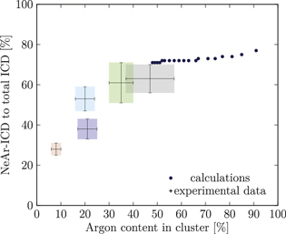
Figure A7.
 ,
,  and SNe= 1–19.
Download figure:
Standard image High-resolution image
Figure A8.
 ,
,  and SNe = 1–19.
Download figure:
Standard image High-resolution imageA.3. Covered surfaces, , and


Figure A9.
 ,
,  and SNe = 1–19.
Download figure:
Standard image High-resolution image
Figure A10.
 ,
,  and SNe = 1–19.
Download figure:
Standard image High-resolution image
Figure A11.
 ,
,  and SNe= 1–19.
Download figure:
Standard image High-resolution image
Figure A12.
 ,
,  and SNe = 1–19.
Download figure:
Standard image High-resolution imageA.4. Covered surfaces, , and


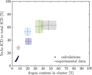
Figure A13.
 ,
,  and SNe = 1–19.
Download figure:
Standard image High-resolution image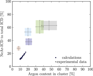
Figure A14.
 ,
,  and SNe = 1–19.
Download figure:
Standard image High-resolution image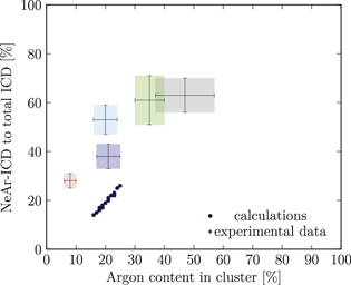
Figure A15.
 ,
,  and SNe = 1–19.
Download figure:
Standard image High-resolution image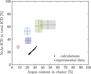
Figure A16.
 ,
,  and SNe = 1–19.
Download figure:
Standard image High-resolution imageA.5. Caps, ,


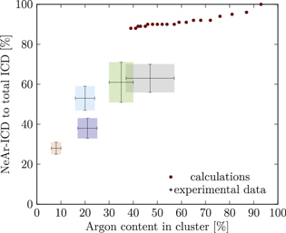
Figure A17.
 , caps = 1–20.
Download figure:
Standard image High-resolution image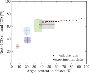
Figure A18.
 , caps = 1–20.
Download figure:
Standard image High-resolution image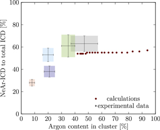
Figure A19.
 , caps = 1–20.
Download figure:
Standard image High-resolution image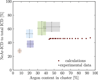
Figure A20.
 , caps = 1–20.
Download figure:
Standard image High-resolution imageA.6. Randomly arranged neon atoms, , and R according to the experiment


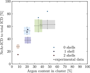
Figure A21. Random arrangements with  and CNe = 0–2.
Download figure:
Standard image High-resolution image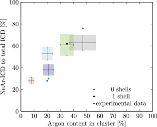
Figure A22. Random arrangements with  and CNe = 0–1.
Download figure:
Standard image High-resolution image
Figure A23. Random arrangements with  and CNe = 1–2.
Download figure:
Standard image High-resolution image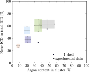
Figure A24. Random arrangements with  and CNe = 1.
Download figure:
Standard image High-resolution image