


Abstract
In cells, dynamic microtubules organize into asters or spindles to assist positioning of organelles. Two types of forces are suggested to contribute to the positioning process: (i) microtubule-growth based pushing forces; and (ii) motor protein mediated pulling forces. In this paper, we present a general theory to account for aster positioning in a confinement of arbitrary shape. The theory takes account of microtubule nucleation, growth, catastrophe, slipping, as well as interaction with cortical force generators. We calculate microtubule distributions and forces acting on microtubule organizing centers in a sphere and in an ellipsoid. Positioning mechanisms based on both pushing forces and pulling forces can be distinguished in our theory for different parameter regimes or in different geometries. In addition, we investigate positioning of microtubule asters in the case of asymmetric distribution of motors. This analysis enables us to characterize situations relevant for Caenorrhabditis elegans embryos.
Export citation and abstract BibTeX RIS

Content from this work may be used under the terms of the Creative Commons Attribution 3.0 licence. Any further distribution of this work must maintain attribution to the author(s) and the title of the work, journal citation and DOI.
1. Introduction
Microtubule asters are cellular structures formed by radial arrays of microtubules nucleated from an organizing center, with microtubule plus ends pointing to the cell boundary. The function of microtubule asters is generally considered as to help the organizing center find its correct position inside the confining space of various shaped cells [1]. Positioning of microtubule asters is achieved by distinct mechanisms in different cells. In the fission yeast Schizosaccharomyces pombe, centering of the nucleus during interphase is governed by pushing forces generated by microtubules polymerizing against the cell cortex [2–4]. In animal cells, cytoplasmic dynein, a minus-end motor protein, mediates pulling forces on the cell cortex that play an important role in the positioning of centrosomes and spindles. For instance, in a single-cell-stage Caenorrhabditis elegans (C. elegans) embryo, asymmetric positioning of the mitotic spindle results from the asymmetric activity of cortex-anchored dyneins [5–7]. Moreover, pulling forces generated by cortical dyneins are also responsible for spindle oscillations that occur during asymmetric spindle positioning [8–10]. Such spindle oscillations require a restoring force generated by a centering mechanism. This force can be characterized by a centering stiffness [8]. Recent studies have shown that a ternary complex LIN-5-GPR-1/2-G, which is responsible for anchoring dyneins to the cortex, is critical for correct positioning of mitotic spindles in C. elegans embryo [11]. Another ternary complex [NuMA]-LGN-G of the same function has also been found in human cells [11, 12]. This demonstrates that dynein-dependent cortical pulling forces, at least in part, control the spindle positioning in these cells. In other cells, such as sea urchin and amphibian eggs or in mammalian cells, pulling forces, generated by dynein motors and acting on microtubules, are also essential for the centering of centrosomes [13–16] and for the alignment of mitotic spindles along the long axis of the cell [17–19]. Recently it has been suggested that dyneins could also generate pulling forces via friction associated with the transport of organelles along the microtubules lateral surface [14, 15, 20]. In general, cells with different geometries or sizes may use different strategies to accomplish the correct positioning of organizing centers.
Both pushing and pulling forces have been suggested to contribute to the positioning of microtubule asters. The force velocity relation of growing microtubules against a rigid object has been determined in vitro [21]. It was also shown that dynein motors can capture microtubule ends and exert pulling forces [22, 23]. Two key mechanisms have been proposed to explain the ability of pushing forces to position the organizing center to the center of a cell: (i) there are more microtubules pushing against the boundary proximal to the organizing center than that distal to the organizing center due to microtubule length distributions resulting from microtubule dynamic instability [24]; and (ii) shorter microtubules can generate larger pushing forces than longer microtubules before they buckle [25]. A centering mechanism based on pulling forces associated with friction due to organelle transport along the microtubule lattice relies on the fact that longer microtubules give rise to larger forces [19, 26]. However, pulling forces generated at microtubule tips can also lead to centering forces if more microtubules are pulling from the side distal to the organizing center. This can happen when there are only a limited number of force generators interacting with microtubule tips [27] or when microtubules reorient toward the distal side of the organizing center after they touch and briefly slip along the cell boundary [22]. We have recently shown that the effects of pushing and pulling forces depend on cell geometry and on the degree of microtubule slipping [22, 28]. In a single elongated geometry, pulling and pushing forces may play different roles along the long and short axes [28].
Our work is an extension of previous work where centering by pushing and pulling forces was discussed in relation to experiments on microtubule asters in artificial microchambers [22, 28]. Here, we develop a general framework that applies to one, two and three dimensions. Our previous work is extended in several ways: we now include effects of microtubule catastrophes before they reach the cell boundary. Such catastrophes help pushing forces to result in stable centering. We now also take the force–velocity relation of pushing microtubules into account, in addition to the effects of length dependent microtubule buckling. We obtain analytical expressions for centering stiffness by pushing and pulling forces in a sphere and a circle and in one dimension. Finally, we discuss asymmetric distributions of force generators that can induce a positioning of the spindle away from the center. We can relate this asymmetric situation to asymmetric spindle positioning in the C. elegans embryo.
2. Mechanics of microtubule asters in a three-dimensional confinement
In our description of microtubule aster mechanics, microtubules are nucleated from an organizing center at a fixed position r that is confined in a volume bounded by a curved surface. This boundary surface is parameterized as R(u1,u2), where u1 and u2 are two parameters. The vector L(u1,u2) = R(u1,u2) − r extends from the organizing center to the boundary, with L = |L| denoting the distance between them, and  the unit vector defining the microtubule orientation (figure 1). We define the metric tensor gij = ei·ej, i, j = 1,2, and its determinant g = det (gij), where ei = ∂R/∂ui are the tangent vectors. The unit vector normal to the boundary is given by m = ± (e1 × e2)/|e1 × e2|, where the sign is chosen that the vector is pointing outward.

Figure 1. Schematic representation of a microtubule aster in a confinement of arbitrary shape. The blue dot represents the organizing center located at position r and the gray mesh represents the boundary R of the confinement. The tangential vectors at the surface are denoted by e1 and e2 and the normal vector is denoted by m. Three microtubules are shown as green rods. The short microtubule with the microtubule tip at the position q inside the confinement represents a cytoplasmic microtubule. The other two microtubules are in contact with the boundary. Inset 1 shows a pulling microtubule that is captured by a cortical force generator (magenta). Inset 2 shows a pushing microtubule that is slipping on the boundary at a velocity v∥. The arrows indicate the direction of the force acting on the microtubule end.
Download figure:
Standard image High-resolution imageWe distinguish three populations of microtubules: (i) cytoplasmic microtubules that have not touched the boundary; (ii) microtubules that are in contact with the boundary and pushing against it; and (iii) microtubules that are in contact with the boundary and pulled by force generators. Cytoplasmic microtubules are described by the volume density distribution of microtubule tips ρ(q) at position q. The equation that governs the evolution of ρ(q) reads

where ν0 denotes the nucleation rate of microtubules from the organizing center, δ3(q) is the three-dimensional Dirac delta function and kcat denotes the catastrophe rate of microtubules in the cytoplasm. The current density of microtubule tips reads J(q) = ρ(q)vgb(q), where vg denotes the microtubule's growing velocity in the cytoplasm, and b(q) = (q − r)/|q − r| denotes the unit vector pointing in the direction of the microtubule. Pushing and pulling microtubules are described by their surface densities, n+(u1,u2) and n−(u1,u2,). The number of pushing and pulling microtubules in contact with the boundary within an area element dS = g1/2 du1 du2 is n± dS. These densities obey the following equations:


Here kc denotes the catastrophe rate of pushing microtubules at the boundary, kb denotes the binding rate of pushing microtubules to the force generators and koff denotes the detachment rate of pulling microtubules from the force generators. The source term, m·J|R = m(u1,u2)·J(R(u1,u2)), in equation (2) describes the flux of arriving cytoplasmic microtubules at position R(u1,u2) on the boundary where they start pushing. The pushing force drives microtubule slipping at the boundary and the slipping is described by the surface current j = n+v∥, where v∥ is the slipping velocity. The covariant divergence of the surface current is D·j = ∂i(g1/2ji)g−1/2, where ji = j·ei are the contravariant components of the vector j and ei is the dual vector of ei. The slipping velocity and the pushing force are related by

where ξ is the friction coefficient associated with slipping and f+∥ = f+ − (f+·m) m is the tangential component of the pushing force  . The surface current of microtubule tips j = n+v∥ then reads

If a microtubule grows against the boundary, it generates a pushing force  in the direction of the microtubule. The growth rate dlm/dt of the microtubule depends on the polymerization force fP, where lm denotes the length of the microtubule [21]. For simplicity, we describe this dependence by a linear force velocity relationship

For straight microtubules, the slipping velocity and the growth rate of microtubules are related by dlm/dt = v∥·L. Combining this relation with equations (4) and (6), we obtain the magnitude of the pushing force f+ = fP as

Equations (1)–(3) together with the surface current j given by equations (5) and (7) define the dynamic equations for the microtubule distribution.
To determine the force acting on the microtubule organizing center, we solve equations (1)–(3) at steady state ∂tρ = 0,∂tn± = 0 to obtain the surface density of pushing microtubules and pulling microtubules n+ and n−. We impose the condition that the total number of the three populations of microtubules is a constant M, which sets the value of the nucleation rate ν0 (appendix A). The net force acting on the organizing center located at position r is given by F(r) = F+(r) + F−(r), where

are the net pushing and pulling forces, respectively. The magnitude of the pulling force is denoted by f−. The direction of pulling forces is along the microtubule's orientation  and the direction of pushing forces is in the opposite direction
  .
.
The net forces acting on organizing centers at different positions r define a force field F(r). The gradient of this force field is given by the stiffness tensor Tαβ = ∂βFα, where α,β = x,y,z label the components of the tensor in Cartesian coordinates. The stiffness tensor Tαβ = −Sαβ + Aαβ can be split into a symmetric part Sαβ and an antisymmetric part Aαβ, where

The eigenvalues of the symmetric tensor Sαβ describe the effective stiffness along directions defined by the eigenvectors. The antisymmetric tensor Aαβ describes the local rotation of the force field. In the case that Aαβ = 0, the force field is conservative and can be written as the gradient of a potential F(r) = −∇Φ, where  and r0 is an arbitrary point inside the confinement. However, in general the antisymmetric tensor Aαβ is nonzero and the force field is nonconservative.
So far we have ignored microtubule buckling. If the microtubule polymerization force fP exceeds the buckling force fE = π2κL−2, where κ denotes the bending rigidity, the magnitude of pushing forces is limited by fE. This effect can be described by choosing

Using equation (10) for the magnitude of pushing force f+ in equations (5) and (8), we can calculate the net force F(r) taking into account effect of microtubule buckling.
Equations (1)–(9) constitute a general description of microtubule aster mechanics inside a three-dimensional confining space. In the following, we apply our theory to different geometries to illustrate the impact of microtubule dynamics or motor distributions on the positioning behavior of microtubule asters. We choose sphere and ellipsoid because these two geometries are of great biological relevance.
3. Mechanics of microtubule asters in a sphere
We first consider microtubule asters confined in a sphere of radius R0. From equations (2) and (3) we determine the microtubule distribution for an organizing center displaced from the sphere center by a distance z along the z-axis (figure 2(A)). Resulting microtubule distributions have rotational symmetry with respect to the z-axis. The direction of microtubules is described by a unit vector  , parameterized by two angles θ and ϕ. Detailed calculations in this (θ,ϕ) coordinate are shown in appendix B. It is convenient to introduce the number of microtubules per solid angle σ = ndS/dΩ, where dΩ = sin θ dθ dϕ is the solid angle element and n = n+ + n−.
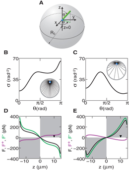
Figure 2. The microtubule distribution and forces acting on an organizing center in a sphere. (A) The coordinate system used to describe the angular distribution of microtubules in a sphere. (B), (C) The angular distribution of microtubules for an organizing center displaced 10 μm from the center. The cytoplasmic catastrophe rate is kcat = 0.001 s−1 in (B) and kcat = 0.1 s−1 in (C). (D), (E) Forces acting on a microtubule organizing center along the z-axis. The pushing (magenta), pulling (green) and net (black) forces on the organizing center are plotted at different positions along the z-axis. The black triangle indicates the 10 μm displacement used for drawing the microtubule distributions. The white quadrants indicate a force pointing toward the center and the gray quadrants indicate a force pointing away from the center. The cytoplasmic catastrophe rate is kcat = 0.001 s−1 in (D) and kcat = 0.1 s−1 in (E). The radius of the sphere is 15 μm. Other parameters are listed in table 1, with kc = 0.5 and kb = 0.25 s−1.
Download figure:
Standard image High-resolution imageTypical distributions of microtubules are shown in figures 2(B) and (C). For small cytoplasmic microtubule catastrophe rate kcat, almost all microtubules reach the boundary. In this case, microtubules are concentrated at the boundary farther from the microtubule organizing center where π/2 < θ < π, which is referred to as the distal boundary (figure 2(B)). At the boundary closer to the microtubule organizing center where 0 < θ < π/2, which is referred to as the proximal boundary, the density σ is lower (figure 2(B)). This angular distribution is the result of microtubule reorientation, which occurs due to microtubule slipping along the sphere surface. For increased cytoplasmic catastrophe rate kcat, the number of microtubules reaching the boundary decreases with increased distance between the organizing center and the cell boundary. This leads to less microtubules arriving at the distal boundary. Therefore, for sufficiently large cytoplasmic catastrophe rate kcat, the microtubule distribution will be inversed and there will be more microtubules touching the proximal boundary than the distal boundary (figure 2(C)).
Different microtubule distributions result in different net pulling and pushing forces acting on the organizing center. If more microtubules are contacting the distal boundary as compared to the proximal boundary, more microtubules are also pulling from the distal boundary. Because at steady state, the surface density of pulling microtubules and pushing microtubules are related by koffn− = kbn+. The fraction of each population of microtubules is fixed. The net pulling force is thus oriented toward the distal boundary, i.e. toward the center (figure 2(D), green line). By contrast the net pushing force is directed away from the center due to more microtubules pushing against the distal boundary (figure 2(D), magenta line). Note that if the buckling effect is taken into account, pushing forces can also be centering, as will be discussed later. If more microtubules are touching the proximal boundary as compared to the distal boundary, pulling and pushing forces exchange their roles (figure 3(E)).
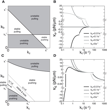
Figure 3. Stability diagram of microtubule asters at the center of a sphere. (A) The stability of microtubule asters at the center of a sphere as a function of the cortical catastrophe rate kc and motor binding rate kb is shown, with white regions indicating that asters at the center are stable and gray regions indicating that asters at the center are unstable. Texts in each panel indicate the stability and the dominating forces. (B) Values of the stiffness for the net force κP at different motor binding rates kb. Values of κP are plotted at different scales separated by the symbol ≈. For kb = 0.1 s−1, the stiffness is a constant zero. Results in (A) and (B) are obtained by using the polymerization force f+ given by equation (7). (C) The same plot as in (A) but the results are obtained by describing the pushing force with the buckling force fE = π2κL−2. Two dashed lines indicate the boundary where values of the stiffness for the pushing force κ+E = 0 and for the pulling force κ−E = 0. (D) The same plot as in (B) but the results are obtained by describing the pushing force by the buckling force. The radius of the sphere is 15 μm. Other parameters are listed in table 1.
Download figure:
Standard image High-resolution imageOur calculations thus reveal that the magnitude and the direction of net pushing and pulling forces depend on the relative strength of microtubule catastrophe in the cytoplasm and microtubule slipping at the boundary. To reveal the role of all the parameters on the forces, we calculate the stiffness tensor Tαβ at r = 0. Because the force field has spherical symmetry and is thus pointing in the radial direction, the antisymmetric part Aαβ of the stiffness tensor vanishes and the symmetric part Sαβ = κPδαβ is isotropic. Here δαβ denotes the Kronecker delta symbol and κP denotes the stiffness. We find that κP = κ+P + κ−P, where


are the stiffness related to pushing and pulling forces, respectively (appendix C). Here τP = R0ξ1/2(fsvg)−1/2 is a characteristic time which is the geometric mean of the duration it takes for microtubules to grow from the center to the boundary and to slide the same distance along the boundary. The parameter d with d = 3 is the space dimension.
Asters can be either stable with κP > 0 or unstable with κP < 0 in the center and aster positioning can be dominated by either pulling or pushing forces. The combination of these possibilities gives rise to four regions in the stability diagram shown in figure 3(A) as a function of motor binding rate kb and microtubule cortical catastrophe rate kc. Different regions are separated by straight lines along which κP = 0. One of the lines is kb = k*b with arbitrary kc, where k*b = kofffs/f−. This line separates regions where pulling forces are dominant from regions where pushing forces are dominant. The second line is kb + kc = k*, where k* = 2(kcatτ2P)−1. This line separates regions where pulling forces pointing toward the center and pushing forces pointing away from the center (κ−P > 0,κ+P < 0) from regions where the direction of pushing and pulling forces are opposite (κ−P < 0,κ+P > 0). Two limiting cases can be discussed: (i) if the microtubule cytoplasmic catastrophe is zero, kcat = 0, centering is only mediated by pulling forces. In this case, centering is stable if kb > k*b independent of kc and unstable if kb < k*b. (ii) If microtubule cytoplasmic catastrophe is sufficiently frequent, kcat > 2f−(fskoffτ2P)−1, centering is only mediated by pushing forces. In this case, centering is stable if kb + kc > k* and kb < k*b and unstable if kb + kc < k* or kb > k*b. To further understand the impact of parameters on the centering stiffness, we plot in figure 3(B) the magnitude of the stiffness as a function of kc for different kb. The stiffness κP changes from large and positive values to small and negative values as the cortical catastrophe rate kc increases, for large enough binding rate, kb > k*. This shows that a small cortical catastrophe rate kc is required to generate large centering stiffness by pulling forces.
We now discuss the effect of buckling. Buckling becomes important if the polymerization force fP given in equation (7) exceeds the buckling limit fE. This happens for large cells with radius R0 > πκ1/2bf−1/2s, because in the vicinity of the sphere center z ≪ R0, the polymerization force (7) fP = fs + O(z2) and the buckling force fE = fE0(1 + 2z cos θR−10) + O(z2), where fE0 = π2κR−20 is the buckling force for a microtubule with a length of the sphere radius R0. For a large sphere, R0 > πκ1/2bf−1/2s, the pushing force acting on the organizing center in the vicinity of the sphere center will be limited by the buckling force. In this case, the centering stiffness associated with pushing and pulling forces are


where τE = R0ξ1/2(fE0vg)−1/2. In the diagram describing stability of centering for the case of equations (13) and (14), there is one region where positioning of asters at the sphere center is stable (figure 3(C)). Within this region there is a sub-region where both pushing and pulling forces lead to centering (κ−E > 0,κ+E > 0). This happens when more microtubules are touching the distal boundary than the proximal boundary, and thus pulling forces alone are stably centering. However, because the anisotropy of microtubule distribution is weak in this case, the pushing force exerted by a smaller number of shorter microtubules in contact with the proximal boundary is still larger than the pushing force exerted by more and longer microtubules in contact with the distal boundary. Therefore the pushing forces alone are also stably centering. The effect of buckling forces on the magnitude of the stiffness is shown in figure 3(D). We find that the overall dependence of κE on kb and kc is similar to the κP in figure 3(B). Their difference mainly occurs for small kb for which the pushing force plays an important role in positioning. The stiffness κ+E related to pushing forces, compared to the stiffness κ+P for which buckling effect is neglected, is strongly enhanced. This is reflected in figure 3(D) in which κE becomes positive as kc increases, while κP in figure 3(B) remains negative for the motor binding rate kb = 0.01 s−1.
In situations where the microtubule binding rate to motors kb is varied at the boundary, corresponding for example to an asymmetric distribution of motors at the boundary, microtubule asters might be displaced away from the center. A typical example is that a large number of motors are located on one side of the sphere, and on the opposite side the motor density is low. To investigate the positioning of microtubule asters in this case, we calculate the net force acting on the organizing center with a spatially varied binding rate kb(θ) = (kP + kA)/2 + (kP − kA)(z + L cos θ)(2R0)−1 where kP and kA are the binding rates at two points at opposite sides on the sphere. For kP ≠ kA, the center of the sphere is no longer a stationary, force-free position. Using parameter values for which the positioning is stable and dominated by pulling forces in the symmetric case, kP = kA, positioning is also stable, but at a location with a distance z = Δ from the center for kP ≠ kA (figure 4(B)) and closer to the boundary where the binding rate is larger. The distance Δ of stable positions of the organizing center as a function of kP/kA is shown in figures 4(C) and (D). We find that for increased cortical catastrophe rates, corresponding to reduced slipping, displacements Δ are increased. This is because without slipping, pulling microtubules will concentrate at the boundary with larger binding rate and pushing microtubules will concentrate at the boundary with lower binding rate. This distribution always creates a force pointing toward the boundary with the larger binding rate. Thus the microtubule organizing center will be positioned to the boundary with the larger binding rate. Microtubule slipping reduces this decentering effect and allows a force-free position with a small displacement Δ. Compared with kc, kP has smaller impact on the displacement (compare figures 4(C) and (D)). But for increasing values of kP, the stiffness at the force-free position decreases (compare the orange and blues line in figure 4(B)). This also happens in the symmetric case for large binding rate kb.
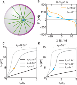
Figure 4. Displacement of microtubule asters from the center of a sphere in the case of spatially asymmetric binding rates. (A) Schematic illustration of the spatially asymmetric binding rate and the resulting microtubule aster displacement. The increasing brightness of the layer (magenta) at the boundary from left to right indicates the increasing binding rate. (B) Forces acting on organizing centers along the z-axis of a sphere. The point where the net force is zero corresponds to the displacement. The binding rate kP = 0.5 s−1 for the orange curve and kP = 5 s−1 for the blue curve. (C), (D) The displacement of organizing centers as a function of the ratio of kP and kA. The orange and blue dots correspond to the displacement obtained from the orange and blue curves in (B), respectively. The radius of the sphere is 15 μm. Other parameters are listed in table 1 with kP = 0.5 s−1 for (B) and kP = 5 s−1 for (C).
Download figure:
Standard image High-resolution image4. Comparison with one and two dimensional confinement
We can also discuss stabilities of asters in the center of lower dimensional confinement. The centering stiffness related to pushing and pulling forces in a circle or in a one-dimensional geometry also obeys equations (11)–(14), with d = 2 for a circle, and d = 1 for a one-dimensional geometry. The stability diagram for a circular geometry is the same to that in a sphere in figure 2, except that k* = (kcatτ2P)−1, which is half of the value of k* for a sphere, while k*b remains the same. This means that the region where asters are stable and positioning is dominated by pulling forces is reduced in d = 2 as compared to d = 3. This is related to the fact that slipping only occurs along a line on a circle. Thus the microtubule anisotropy induced by microtubule reorientation is weaker for a circle as compared to a sphere where slipping occurs in two dimensions. For a one dimensional confinement d = 1, k* becomes zero while k*b does not change. In the stability diagram, centering of microtubule asters is stable if kb < k*b, and unstable if kb > k*b. This means only pushing forces can center the microtubule aster, as suggested in [24, 29].
5. Mechanics of microtubule asters in an ellipsoid
In order to study the role of the shape of the geometry, we apply our general theory, given in section 2, to investigate positioning of microtubule asters confined in an ellipsoid. An ellipsoid, with semi-axes (a,a,a(1 + γ)), has lower symmetry than a sphere. Here γ is a parameter which is zero for a sphere and nonzero for an ellipsoid. The number of microtubules per solid angle σ can be expressed with two angles, σ = σ(θ,ϕ) (figure 5(A)). We limit our study to the case γ > 0 in which the long axis of the ellipsoid is along the z-axis. We find that the distribution of microtubules exhibits different features for organizing centers placed along the z-axis and along the x-axis of the ellipsoid. Along the z-axis, when the organizing center is slightly displaced from the center, microtubules are concentrated at the two poles where θ = 0 or π, while they are depleted for intermediate angles (figure 5(B)). However, if the organizing center is displaced far from the center, microtubules are depleted at the pole for θ = 0 (figure 5(C)). For displacements along the x-axis, microtubules are concentrated at positions that are the farthest from the organizing center, irrespective whether the displacement of the organizing center is large or small. This concentration corresponds to peaks of σ as a function of θ for ϕ = π (figure 5(D), blue line).

Figure 5. The microtubule distribution and forces acting on an organizing center in an ellipsoid. (A) The coordinate system used to describe the angular distribution of microtubules in an ellipsoid. (B)–(D) The angular distribution of microtubules. The displacement of the organizing center is 5 μm in (B) and 20 μm in (C) along the z-axis, 7.5 μm in (D) along the x-axis. Inner figures show the angular distribution of microtubules in a schematic way. (E), (F) Forces acting on microtubule organizing centers in an ellipsoid. The pushing (magenta), pulling (green) and net (black) forces are plotted at different positions along the z-axis (E) and the x-axis (F). The black triangle indicates the position used for drawing the microtubule distributions. The above letters indicate the subfigures showing the corresponding distribution in (B)–(D). The white quadrants indicate a force pointing toward the center and the gray quadrants indicate a force pointing away from the center. Lengths of the three principal axes (x,y,z) of the ellipsoid are 30 μm, 30 μm and 50 μm. Other parameters are listed in table 1, with kb = 0.25 s−1 and kc = 0.5 s−1.
Download figure:
Standard image High-resolution imageDistinct features of microtubule distributions for organizing centers placed along the long axis and the short axis lead to different force behaviors along these two axes. The difference is characterized in figures 5(E) and (F) where the forces acting on organizing centers along the two axes are shown for an ellipsoid with γ = 2/3. Using parameters listed in table 1, we find that along the long axis, in the vicinity of the center, forces due to pulling are weaker than forces due to pushing even though there are more pulling microtubules than pushing microtubules. This is because microtubules concentrate at both sides (θ = 0 and π, figure 5(B)). Pulling forces from the two sides have the same magnitude and are thus almost balanced, while pushing forces generated by microtubules in contact with the proximal side have larger magnitude than microtubules in contact with the distal side. However, for an organizing center far from the center, forces due to pulling are stronger than forces due to pushing. This is because of the accumulation of microtubules at the distal side (θ = π) and depletion of microtubules at the proximal side (θ = 0). Along the short axis, forces due to pulling point toward the center while forces due to pushing point away from the center, regardless of the distance of the organizing center from the ellipsoid center. This is because microtubules accumulate at the opposite side of the displacement of organizing centers. Note that if buckling is considered, the pushing force may point toward the center as well.
Table 1. List of parameters.
| Parameters | Value | Source |
|---|---|---|
| Detachment rate of microtubules from force generators | koff=0.1 s−1 | [8] |
| Growth velocity of microtubules | vg=1 μm s−1 | [33] |
| Pulling force generated by force generators | f−=5 pN | [22] |
| Microtubule stalling force | fs=5 pN | [21] |
| Microtubule bending rigidity | κb=30 pN μm2 | [25] |
| Number of microtubules | M=2000 | [30] |
| Catastrophe rate of microtubules in the cytoplasm | kcat=0.001 s−1 | [10]a |
| Sliding friction coefficient of microtubules | ξ=1 pN s μm−1 | [34]b |
aEstimation from the reported rarely occurred cytoplasmic catastrophe events. bCalculated as the rotational friction of a cylinder of length 15 μm and diameter 25 nm in a viscous media that has 100 times the viscosity of water.
Forces acting on microtubule organizing centers behave differently in a sphere and in an ellipsoid. One difference is that the symmetric part Sαβ (r = 0) of the stiffness tensor, which is isotropic in a sphere, becomes anisotropic in an ellipsoid due to the broken symmetry. In detail, Sαβ (r = 0) is a diagonal matrix, with the stiffness component along the long axis Szz = κL and along the short axis Sxx = Syy = κS. We distinguish contributions to the stiffness from the pushing force, denoted by κ+L and κ+S, and from the pulling force, denoted by κ−L and κ−S. The value of these stiffness components varies as the shape changes from a sphere to an ellipsoid, i.e. the elongation parameter γ increases from zero to positive values (figure 6). Along the long axis, κ+L increases from negative values to positive values and then decreases. At a point for which κ+L = κ−L, contributions from the two types of forces are equal, and beyond which the pushing force becomes stronger than the pulling force (figure 6(A)). We have discussed such a situation in figure 5. However, along the short axis, κ+S remains negative and κ−S remains positive, as in the case of a sphere for all γ. Note that κ+S can be positive if buckling effects are considered. Another difference between forces acting on organizing centers in an ellipsoid and in a sphere is that the force field F(r), which is conservative in a sphere, becomes nonconservative in an ellipsoid (figure 7(A)). In order to see this, we calculate the antisymmetric part Aαβ of the stiffness tensor. Because of symmetry, the components Axy,Ayx,Ayz,Azy of the antisymmetric tensor vanish, and the remaining components Axz = (∂zFx − ∂xFz)/2 and Azx = −Axz are related to the vorticity of the force field ω = ∇ × F by the equation ω = 2Axzey. We find that the vorticity has the largest magnitude in the neighborhood of the two poles of the ellipsoid with γ = 2/3 (figure 7(B)). In regions where xz < 0, the vorticity is positive, implying clockwise rotation of the force field. While in regions xz > 0, the vorticity is negative, implying counter-clockwise rotation of the force field. These are illustrated in figure 7 where the force field in an ellipsoid and the corresponding vorticity are shown, demonstrating that the force field is nonconservative.
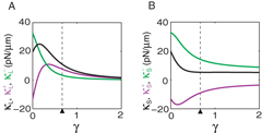
Figure 6. The magnitude of the centering stiffness in an ellipsoid. (A), (B) The magnitude of stiffness as a function the elongation parameter γ along the long axis (A) and along the short axis (B). Contributions to the stiffness from pushing forces (magenta), pulling forces (green) and net forces (black) are shown, respectively. The black triangle indicates the value of γ = 2/3 used in figure 5. Lengths of the three principal axes of the ellipsoid are 30, 30 and 30(1 + γ) μm. Other parameters are listed in table 1, with kb = 0.25 s−1 and kc = 0.5 s−1.
Download figure:
Standard image High-resolution image
Figure 7. Force field in an ellipsoidal geometry and the vorticity of the force field. (A) The force field F(r) in the plane y = 0. Lengths of arrows indicate the magnitude of the forces. (B) Magnitude of the vorticity of the force field ω = ∇ × F(r). Positive values correspond to rotation around the y-axis (clockwise) and negative values correspond to rotation around the −y-axis (counterclockwise). Lengths of the three principal axes (x,y,z) of the ellipsoid are 30, 30 and 50 μm. Parameters are listed in table 1, with kb = 0.25 and kc = 0.5 s−1.
Download figure:
Standard image High-resolution image6. Discussion
In this paper, we presented a general theory for the mechanics and positioning of a microtubule aster in an arbitrarily shaped confinement. Using differential geometry, we characterized processes taking place at the boundary, including microtubule slipping, catastrophe and interaction with cortical force generators. We investigated how the dynamic properties of microtubules and the geometry of the confinement influence the forces acting on the microtubule organizing center. We showed that in a spherical geometry and a circular geometry, centering of microtubule organizing centers depends on two competing factors: microtubule reorientation at the boundary and microtubule catastrophe in the cytoplasm. Microtubule reorientation leads to overall pulling forces pointing toward the center and overall pushing forces pointing away from the center, while microtubule catastrophe in the cytoplasm has the opposite effect. Thus pulling forces together with microtubule reorientation or pushing forces together with microtubule catastrophe in the cytoplasm contribute to stable centering of microtubule organizing centers. The effect of geometry on the positioning forces was demonstrated by studying asters confined in an ellipsoid. The positioning forces along the long axis behave differently as compared to forces along the short axis. For pulling forces, centering stiffness is high along the short axis. While reliable centering along the long axis is better achieved using pushing forces. We also investigated the influence of the distribution of force generators on the positioning forces. Studying asters confined in a sphere with larger binding rate at one side of the surface as compared to the other, we found that microtubule organizing centers are positioned away from the center at a position closer to the boundary with higher binding rates.
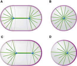
The study of aster positioning in a sphere with asymmetric binding rate can be related to the positioning of mitotic spindles in the C. elegans embryo. A mitotic spindle consists of three types of microtubules. Between the two spindle poles, kinetochore microtubules and polar microtubules form a relatively rigid bundle structure. Astral microtubules are mainly located in the two half-spheres of the oval-shaped embryo (figure 8(A)). Therefore, for simplicity we consider the mitotic spindle in the C. elegans embryo to be structurally analogous to a single microtubule aster in a sphere. In this simplification, the two spindle poles are represented by a single pole and the orientation of the spindle is ignored (see figures 8(A) and (B)). Experiments have shown that the midpoint of the two spindle poles, separated by a distance of around 20 μm, is displaced approximately 4 μm from the cell center along the 50 μm-long anterior–posterior axis during anaphase [9]. This displacement has been suggested to be the result of 50% more force generators at the posterior cortex than at the anterior cortex [7]. Asymmetric distribution of force generators at the cortex corresponds in our model to a spatially asymmetric binding rate at the surface (figure 8(C)). Therefore our findings that asters tend to be positioned away from the center of a sphere and closer to the boundary with higher binding rates provides a possible explanation for the asymmetric positioning of mitotic spindles in the C. elegans embryo (see figures 8(C) and (D)).
Figure 8. Schematic diagram of astral and spindle microtubules in a C. elegans embryo and their approximations with a single aster in a sphere. (A) Schematic illustration of microtubule distributions in a oval-shaped geometry with homogenous binding rate at the two-half spheres. Astral microtubules (green rods) extend from two centrosomes (blue dots) and point toward the edge. The central thick rod connecting the two centrosomes represents the mitotic spindle. (B) Approximation of astral microtubules in (A) with a single aster in a sphere. (C) The same plot as in (A) but with spatially asymmetric binding rates at the two-half spheres. The increasing brightness of the layer (magenta) at the two half-spheres from left to right indicates the increasing binding rate. The mitotic spindle is displaced toward the right side. (D) Approximation of the astral microtubules in (C) with a single aster in a sphere displaced away from the center.
Download figure:
Standard image High-resolution image
The parameter values listed in table 1 have been determined by experiments of the C. elegans embryo or have been estimated indirectly. The remaining unknown parameters are kA,kP and kc. Figure 4 showed how the spindle displacement Δ depends on the ratio kA/kP. The observation that the number of force generators at the posterior cortex is 50% more than that at the anterior cortex suggests kP/kA = 1.5. The observed displacement Δ = 4 μm is consistent with kc = 0.5 and 0.5 s−1 < kP < 5 s−1 (figures 4(C) and (D)). However, we found that the stiffness of positioning is higher for kP = 0.5 s−1 as compared to kP = 5 s−1, which suggests spindle positioning is more reliable for kP = 0.5 s−1. Considering the uncertainty of the friction coefficient ξ (ten times within the value in table 1), we estimate kc lies between 0.05 and 5 s−1. This is consistent with the precision estimated in the existing literatures [10].
In this work we have not considered the fact that cortical binding sites might be saturated by the high density of microtubules reaching the cortex. This fact could also lead to a centering mechanism of microtubule asters by pulling forces [27]. We can incorporate this mechanism in our theory by a density dependent microtubule binding rate kb(n−) = k0b(1 − n−/nmax), where nmax denotes the saturated surface density of pulling microtubules, k0b denotes the binding rate if all binding sites are empty. The resulting equations are nonlinear with respect to the surface densities.
The results of this work correspond to a mean-field description. They characterize the average behavior of centering if many instances of the system are realized. Here we do not include a discussion of fluctuations which can become important when the number of microtubules is small. However in a C. elegans spindle there are more than a 1000 microtubules and the system behaves reliably [30]. Here, we have only considered the case where the cortical catastrophe rate kc is force independent. Taking a possible force dependence of this rate into account, as shown in vitro and in vivo [31, 32], will change the time that microtubules contact the boundary and thus changing the net force. This, however, does not change our results of the centering stiffness equations (11) and (12) in a sphere for which the pushing force is caused by microtubule polymerization. Because the polymerization force fP = fs + O(z2) in the vicinity of the sphere center for z ≪ R0, and the second order contribution does not influence the stiffness derived from linear analysis. On the contrary, the force-dependent catastrophe rate might change our results of the centering stiffness equations (13) and (14) for which the pushing force is caused by microtubule buckling. Investigation of these effects will be our future effort.
In summary, our work provides a theoretical framework to investigate positioning mechanisms of microtubule asters in a confined geometry. The theory allows us to predict the force acting on microtubule organizing centers in an arbitrarily shaped cell for given dynamical properties of microtubules. These predictions, together with future experiments, will help elucidate the positioning mechanisms of microtubule asters in different cell types.
Acknowledgments
We thank David Zwicker for critical reading of the manuscript and Ivana Šarić for drawing the figures. LL gratefully acknowledges support from Human Frontier Science Program.
Appendix A.: Steady state nucleation rate
The nucleation rate ν0 is determined by the condition that the total number of microtubules extended from the organizing center is a constant M at steady state ∂tρ = ∂tn+ = ∂tn− = 0. Note that equations (1)–(3) have the scaling property that if ρ,n+,n− are the solutions for a given nucleation rate ν0, then λρ,λn+,λn− are the solutions for the nucleation rate λν0. Therefore we can choose a particular nucleation rate, for instance, ν*0, and calculate the corresponding solutions ρ*,n+*,n−*. The total number of cytoplasmic microtubules, pushing microtubules and pulling microtubules is then  . The nucleation rate ν0 that satisfies the condition that the total number of microtubules is M then reads

Appendix B.: Equations (1)–(3) in the spherical coordinate centered at the microtubule organizing center
In order to solve equations (1)–(3), we choose a spherical coordinate system (θ,ϕ), in which the microtubule orientation  is described by
  , and the position q of microtubule tips is described by
  , where l is the distance from the organizing center to the microtubule tip. With l as the variable, equation (1) can be simplified into

Note that for different microtubule orientations specified by (θ,ϕ), ρ(l) is defined on the interval l∈[0,L(θ,ϕ)].
We next express equations (2) and (3) in the spherical coordinate. As the current density of microtubule tips in equation (2) reads J = ρ(l)vgb, the source term in equation (2) in the (θ,ϕ) coordinate becomes  , where the dot product of the normal vector m and the unit vector of microtubule orientation is
  , with the determinant of the metric tensor g = L4 sin2 θ + L2(∂θL)2sin2θ + L2(∂ϕL)2. The surface current of microtubule tips at the boundary is j = v∥n+, where the slipping velocity of microtubule tips v∥ is given by v∥ = f+∥/ξ. Here the tangential component of the pushing force f+∥ is

where  and
and  are the tangent vectors and eθ and eϕ are the corresponding dual vectors. Thus the θ component of the surface current j reads

where gij = ei·ej, i, j = θ,ϕ. Using equations  and gij = (gij)−1, we obtain

Through similar procedures we can also get the ϕ component of the surface current j,

Note that jθ has the same sign as ∂θL and jϕ has the same sign as ∂ϕL. This implies that microtubules slip toward the direction where the distance between the organizing center and the cell boundary becomes larger. Since in curvilinear coordinate system, the divergence reads  , equations (2) and (3) are transformed into


We use a finite difference method to numerically solve equations (B.1), (B.6) and (B.7) at steady state, ∂tρ = ∂tn± = 0. The resulting force F(r) acting on the microtubule organizing center is then obtained via equation (8).
Appendix C.: Centering stiffness in a sphere
Because the symmetric part Sαβ(r = 0) = κδαβ of the stiffness tensor is isotropic, we show here the derivation of the value of the stiffness  . Assume the organizing center is displaced along the z-axis by a small distance z, due to rotational symmetry around the z-axis, the solution to equations (B.6) and (B.7) is ϕ independent, n±(θ,ϕ) = n±(θ). We expand the distance between the organizing center and the sphere boundary L(θ) as a series of z, L(θ) = R0 − z cos θ + O(z2), as well as the pushing force f+(θ) = f+0(θ) + f+1(θ)z + O(z2). The solution is expanded as series of z as well, n+(θ) = n+0(θ) + n+1(θ)z + O(z2). Substituting these expansions into equation (B.6) and arranging all terms according to the order of z, we get the perturbative solution to the first order


Here we have used the fact that the steady state solution to equation (B.1) is  . According to equation (8), the z component of the pushing force and the pulling force are


The stiffness κ+ = −∂zF+z and κ− = −∂zF−z thus are


For the pushing force described by equation (7), f+ = fs + O(z2). For the pushing force limited by microtubule buckling, f+ = fE0(1 + 2 cos θz/R0) + O(z2). Substituting these expansions and equations (C.1) and (C.2) into equations (C.5) and (C.6), we get the stiffness values expressed in equations (11)–(14).