


Abstract
We employ a nonequilibrium energy balance and carrier rate equation model based on microscopic semiconductor theory to describe the quantum-dot (QD) laser dynamics under optical injection and time-delayed feedback. The model goes beyond typical phenomenological approximations of rate equations, such as the α-factor, yet allows for a thorough numerical bifurcation analysis, which would not be possible with the computationally demanding microscopic equations. We find that with QD lasers, independent amplitude and phase dynamics may lead to less complicated scenarios under optical perturbations than predicted by conventional models using the α-factor to describe the carrier-induced refractive index change. For instance, in the short external cavity feedback regime, higher critical feedback strength is actually required to induce instabilities. Generally, the α-factor should only be used when the carrier distribution can follow the QD laser dynamics adiabatically.
Export citation and abstract BibTeX RIS

Content from this work may be used under the terms of the Creative Commons Attribution 3.0 licence. Any further distribution of this work must maintain attribution to the author(s) and the title of the work, journal citation and DOI.
1. Introduction
The nonlinear dynamics of semiconductor lasers under external optical perturbations have been the subject of extensive experimental and theoretical studies. Of particular interest are the dynamical response of lasers to the injection of an optical signal into the cavity [1–6] and their sensitivity to time-delayed optical self-feedback [7–16].
It is generally accepted that quantum-dot (QD) lasers exhibit less complex dynamics when subjected to optical perturbations [17]. For technological applications QD lasers thus have the advantage of a lower sensitivity to optical feedback [18] when compared to conventional quantum-well (QW) devices. The theoretical discussion of optically perturbed QD lasers is usually carried out on the basis of rate equations. From an analysis of these rate equations, the reduced sensitivity of QD lasers toward perturbations can be attributed to the strong damping of relaxation oscillations (ROs) in QD lasers [18–21] and a smaller amplitude-phase coupling. The amplitude-phase coupling is commonly expressed in terms of the phenomenological linewidth-enhancement factor α [22], assuming a linear relationship between changes of the gain and refractive index in the active laser medium. As we have previously shown [23, 24], the concept of the α-factor can break down in QD lasers, and a more rigorous modeling approach must be used to accurately account for the charge carrier dynamics of all optically active charge carrier states. While a microscopic description of the QD laser dynamics under optical perturbations would be favorable, the large computational effort associated with such an approach generally prevents a thorough bifurcation study.
In this paper, we present a microscopically based balance equation (MBBE) model, consisting of energy balance and carrier density rate equations based on a microscopic laser model. We show that such a model can very well reproduce the predictions of the microscopic model, while still maintaining the computational simplicity of conventional rate equations. We are consequently able to perform a thorough bifurcation analysis of the nonlinear QD laser dynamics when optical injection or time-delayed feedback is considered. We highlight the differences in the QD laser dynamics inferred by using an α-factor when compared to our MBBE model. We can show that, depending on the charge carrier scattering lifetimes, an α-factor will lead to qualitatively different predictions of the laser dynamics. Furthermore, we find that the desynchronized dynamics of refractive index and gain lead to a simplification of occurring dynamical instabilities and reduce the sensitivity of the laser to optical feedback.
The paper is organized as follows. In section 2 we present the theoretical model used to describe the QD laser device with optical injection or time-delayed optical feedback. We then present numerical bifurcation analyses of the laser system under optical injection or feedback in section 3. A conclusion is then given in section 4.
2. Microscopically based balance equation model
We consider a 1.2 mm long ridge waveguide edge-emitting dot-in-a-well single-mode laser device, consisting of a number of aL = 15 stacked InGaAs QW layers with height hQW, each embedding a density of NQD InAs QDs. The QDs are assumed to have localized bound electron and hole states, with a ground state (GS) centered at a transition frequency corresponding to an emission linewidth of λ = 1.3μm, and the twofold degenerate first excited state (ES). Figure 1 illustrates the energetic structure of the device across one QD.
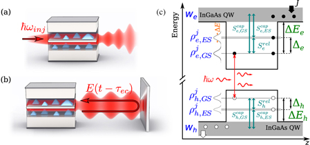
Figure 1. Schematic illustration of the considered QD laser structure with (a) optical injection and (b) time-delayed optical feedback. (c) Energy diagram across one QD. ρjb,m denote the QD occupation probabilities for b = {e,h}, m = {GS,ES} and the subgroup index j of the inhomogeneously broadened QD ensemble, with its spectral width given by ΔE. The QD GS subgroup with  is assumed to match the laser mode energy ℏω. The QDs are embedded in InGaAs QWs, which are electrically pumped (pump strength J). The QW carrier density is given by wb. The QD center ground state (GS) energy lies ΔEb below the QW band edge, with one excited state lying Δb above the GS energy. The charge carrier exchange between different states is described by the direct capture scattering rates Scapb,m, and the relaxation rates Srelb.
Download figure:
Standard image High-resolution imageWe distribute the QD bound states into different subgroups, denoted by the index j, to account for the inhomogeneous broadening of the QD gain material. The probability density function f(j) describes the probability to find a QD in the jth subgroup, assuming a normal distribution of the QD transition energies

where ωjm is the transition frequency of the jth QD subgroup of the mth bound QD state, with m = {GS,ES}, and ω is the cavity resonance frequency. The inhomogeneous broadening width (FWHM) is given by ΔE, and
is a normalization parameter, chosen such that  . The spectral broadening of the QD transitions is given by the sum of the broadening of the electron and hole single-particle energies of the bound GS: ΔE = Δεe + Δεh. We assume a broadening of the bound state energies proportional to the corresponding localization energies:
  . In the simulations, we will use
  for a total of jmax + 1 = 51 subgroups, distributed uniformly in the GS transition energy interval [ℏω − 2ΔE,ℏω + 2ΔE].
The dynamic system describing the laser is modeled within a rate equation approach based on the optical Bloch equations [24–29]. We start with the equations for the slowly varying electric field envelope  , the occupation probabilities in each subgroup of the QD bound state ρjb,m, and the carrier densities in each QW layer wb, given by the sum over all occupation probabilities ρb(k2D) in the two-dimensional (2D) k-states k2D:

with the in-plane device area A. The real electric field is given by ![$E(t)=\frac {1}{2}[{\mathscr{E}}(t){\mathrm { e}}^{-{\mathrm { i}}\omega t}+{\mathscr{E}}^*(t){\mathrm { e}}^{{\mathrm { i}}\omega t}]$](https://content.cld.iop.org/journals/1367-2630/15/9/093031/revision1/nj479513ieqn6.gif) . The index b = {e,h} distinguishes electrons and holes, m = {GS,ES} distinguishes QD ground and first excited states:
. The index b = {e,h} distinguishes electrons and holes, m = {GS,ES} distinguishes QD ground and first excited states:


In the above equations, Γ = aLhQWA/Vmode denotes the geometric confinement factor (Vmode = 10−15 m3 is the effective mode volume), εbg and ε0 are the background and vacuum permittivity, respectively, and κ is the optical loss rate. The sum over α includes all possible optical transitions, where μα and pα are the corresponding dipole transition matrix element and the microscopic polarization, respectively. The spontaneous recombination losses in the QDs are given by the recombination rate Wm. Rwloss describes the charge carrier losses in the QW states due to spontaneous recombination and takes higher order losses into account phenomenologically. J is the pump current density per unit area into the QW states, with the electron charge e0.
Representing details of QD dephasing [30, 31] with an effective dephasing time T2, and assuming that this time is sufficiently short to allow the interband polarization pα to be adiabatically eliminated, yield the quasi-static relation

where Δωα ≡ ωα − ω is the frequency detuning of the transition α. The microscopic polarization thus takes on a value proportional to the electric field, and is modulated by the homogeneous linewidth, given by a Lorentzian line shape with a width of 2ℏ/T2, centered on the cavity resonance frequency, with its imaginary part decaying like (Δωα)−2 and its real part like (Δωα)−1 for large detuning |ΔωαT2| ≫ 1. Inserting the relation for pα given in equation (7) into equation (4), the equation can be rewritten as

where Re[g(ω,t)] describes the amplitude gain of the electric field and Im[g(ω,t)] is the change of instantaneous electric field frequency due to carrier-induced changes of the refractive index. The sum is now separated into the sum over the localized QD states (with νm their degree of degeneracy excluding spin) and the corresponding subgroups, as well as a sum over the QW k-states.
The optical transition frequencies of the QW can be assumed to be detuned far enough from the laser frequency such that they do not influence the amplitude gain appreciably. However, since the real part of the microscopic polarization decays more slowly than its imaginary part, the QW transitions need to be taken into account when determining the instantaneous frequency change of the electric field. In equation (9), this is done by including the contribution of the polarization of the QW transitions pk2D QW to the imaginary part of the complex gain.
The definition of the complex gain in equation (9) shows that every optical transition contributes to gain and index change differently. The total differential changes of these quantities during the operation of the QD laser, which strongly influence the dynamic response to optical perturbations, is thus dependent on the variation of the charge carrier occupation for each independent transition. It is therefore in general not possible to make predictions about the laser dynamics without a careful consideration of the charge carrier dynamics, as we will show later on in section 3, where we compare our results with a model where the ratio of frequency and gain changes are related by a single factor (α-factor).
The scattering terms labeled ∂tρ|col in equations (5) and (6) governing the charge carrier exchange between the carrier reservoir and the QD bound states are written as [32, 33]


where + and − correspond to m = GS and ES, respectively.
Scattering processes in a QD structure can be substantially different from a QW, requiring non-perturbative treatment and memory effects [30, 34, 35]. For the present study, we neglect those differences and revert to the customary second Born and Markov approximation calculations to determine the nonlinear capture rates Sin,cap into the bound QD states as well as the relaxation rate Sin,rel between the QD ES and GS, including their dependences on the QW charge carrier density and temperature [36, 37]. The corresponding out-scattering (escape) rates can be determined from detailed balance relations [33]


where EFbeq and Teqb are the carrier density dependent quasi-Fermi level and quasi-equilibrium temperature of the QW carrier distribution, respectively. The energy spacing between GS and ES is given by Δb. The energy εjb,m denotes the single-particle energy of the jth subgroup of the mth bound QD state, and kB is the Boltzmann constant. Here it is assumed that the QW states are in quasi-equilibrium, i.e. the QW carrier distributions can be described by quasi-Fermi-distributions f(εb(k2D),EFbeq,Teqb). This assumption is supported by simulations of the microscopic model, which shows only very little deviation from quasi-equilibrium within the QW distribution.
Until now, no assumption was made about the charge carrier temperature Teqb. Often, it is assumed to be close to the ambient or lattice temperature. However, in QD optoelectronic devices the charge carrier temperature can exceed the lattice temperature Tℓ, due to carrier heating effects such as free-carrier and two-photon absorption or Auger-heating [38–42]. The reason for Auger-heating is that Auger scattering processes are energy conserving. Thus, whenever a charge carrier scatters from a carrier reservoir state into a energetically lower QD state, another charge carrier will gain the energy difference as kinetic energy, thus leading to a heating of the carrier distribution. This mechanism is illustrated in figure 2 for direct capture and QD carrier relaxation processes. In the microscopic description (see appendix A), the carrier heating can be extracted from the k2D-resolved carrier occupation. This, however, requires the computationally demanding tracking of the carrier occupation of each k2D-state and the numerical solving of energy and carrier conservation conditions in each simulation time step. In our balance equation model, we describe carrier heating effects in the 2D reservoir by means of combined carrier density and energy balance equations [43, 44], allowing us to reproduce the results of the microscopic model without the need to track every k2D-state separately, thus reducing computation time significantly. A similar approach was presented in [42], which we generalize by including the first ES of the QD and going beyond the low-carrier-density limit.
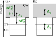
Figure 2. Mechanism of Auger-heating in QD devices, shown representatively for electrons only. (a) Direct capture processes: a carrier with energy ε1 relative to the QW band edge scatters into a QD state, while another carrier gains kinetic energy equal to ΔEme + ε1. The net energy change in the QW is ΔEme. (b) Relaxation processes: a carrier relaxes from the QD ES into the GS, adding a net energy of Δe to the total QW carrier energy.
Download figure:
Standard image High-resolution imageIn order to account for dynamic changes in the charge carrier temperature, we now derive the additional energy balance equation for the QW carriers. The total charge carrier energy density ub per unit area in the QW can be determined from summing over all electronic k-states in the QW:

where εb(k2D) is the single-particle energy of the electronic state at k2D. In quasi-equilibrium, the QW carrier energy density can be expressed via

with the quasi-Fermi distribution f(ε,EF,T). The quasi-Fermi level relative to the QW band-edge in dependence of the QW carrier density wb is given by

with the 2D density of states Db = m*b/(πℏ2) and the sign + (−) for b = e (h). Using the above expression, the carrier energy density can be evaluated as a function of the carrier density and temperature: ueqb(wb,Tb). By solving the inverse function, a corresponding quasi-equilibrium carrier temperature Teqb(wb,ub) can be assigned to each combination of carrier density and energy density in every time step of the simulation.
The QW energy density balance equation can be written in terms of contributions from different sources:

We consider a change in carrier energy due to electrically pumped carriers (subscript pump), interband recombination processes (rec), Auger-scattering (col), scattering with lattice phonons (phon), and due to the thermalization of the electron and hole distributions toward a common carrier temperature (th) [45]. These contributions are given by the following expressions:


Here,  is the average carrier energy of electrically injected carriers, and γp, γth are the carrier–phonon scattering and thermalization rates, respectively. In equation (22) the rhs enters with a negative (positive) sign for electrons (holes). The partial derivatives in equation (20) account for charge carrier scattering between the QW and the QD ground and excited states, as well as relaxation processes between GS and ES, respectively:


2.1. Optical perturbations: optical injection and time-delayed optical feedback
We now consider the optical perturbation of the QD laser system by optical injection and time-delayed optical feedback. In an optical injection setup, an external optical signal, e.g. from a different (master) laser, is injected into the (slave) laser cavity. Assuming a monochromatic external signal, the optical injection leads to an additional forcing term in the electric field equation

Here, the injected signal optical frequency is given by ωinj, and the dimensionless injection strength is K, where E0 is the steady-state electric field amplitude of the free-running solitary laser, and τin is the cavity round-trip time. The injection strength then equals the square root of the injected power ratio,  .
.
Considering the free-running laser in the steady-state, its oscillation frequency is shifted from the carrier frequency ω due to charge-carrier-induced frequency changes. These changes are given by the imaginary part of the gain, such that the free-running laser frequency is given by

where g0 is the steady-state complex gain of the free-running laser, given by equation (9) evaluated at the steady-state. We now define the injection frequency detuning as the frequency difference between the injected signal and free-running laser

In order to eliminate the explicit time-dependence of the injected signal, we express the electric field in a rotating frame [3], given by

Inserting this equation into equation (25) yields

Besides optical injection, time-delayed optical feedback in semiconductor lasers has been a topic of great interest [12, 16, 46–48]. When an external mirror is placed in the laser beam outside of the laser cavity with a distance ℓ, the emitted light couples back into the laser cavity after a time τec = ℓ/c, where c is the vacuum speed of light. We model this by introducing a time-delayed feedback term in the time evolution of the electric field

where C is the phase of the reflected electric field, and Kfb∈[0,1] is the feedback strength, denoting the ratio of the light lost through the cavity mirrors that is coupled back into the cavity. Again, the electric field is expressed in a rotating frame, such that its phase velocity vanishes in the steady-state. The external cavity feedback time τec and the feedback phase C are in principal both determined from the optical path length of the feedback section, however, the feedback phase is much more sensitive to changes. A change of the optical path length of one photon wavelength leads to a complete rotation by 2π of the feedback signal, while τec barely changes. Thus, the feedback phase and delay time can generally be assumed to be independent from each other.
3. Bifurcation analysis
We now employ the model presented in the previous section in numerical simulations. The parameters used in the simulations are given in table 1, unless stated otherwise. In the following, we discuss two different types of QDs, characterized by their localization energies, as given in table 2, which we refer to as shallow and deep QDs, respectively. In the shallow QD structure the localized QD states have a comparably low energetic distance to the QW band edge, which leads to carrier exchange between QD and QW on the order of picoseconds. On the other hand, the deeply confined QDs reduce the scattering efficiency, leading to slower electron scattering on the order of nanoseconds.
Table 1. Numerical parameters used in the simulation.
| Symbol | Value | Symbol | Value |
|---|---|---|---|
| κ | 0.05 ps−1 | τin | 48 ps |
| μm | 0.6 e0 nm | WGS | 0.44 ns−1 |
| μQW | 0.5 e0 nm | WES | 0.24 ns−1 |
| εbg | 14.2 | Rwloss | 540 ns−1 nm2 |
| Γ | 0.15 | ℏω | 0.952 eV |
| T2 | 100 fs | hQW | 4 nm |
| ΔE | 55 meV | NQD | 1011 cm−2 |
| εp,e | 155 meV | m*e | 0.043me |
| εp,h | 76 meV | m*h | 0.45me |
| γp | 1011 s−1 | γth | 1012 s−1 |
| jmax | 51 | A | 2.4×10⁻⁵ cm−2 |
| aL | 15 |
Table 2. QD localization energies for the considered QD structures.
| Shallow dots | Deep dots | ||
|---|---|---|---|
| Symbol | Value | Symbol | Value |
| ΔEe | 74 meV | ΔEe | 210 meV |
| ΔEh | 40 meV | ΔEh | 50 meV |
| Δe | 50 meV | Δe | 64 meV |
| Δh | 20 meV | Δh | 6 meV |
| Im[g0](J=2Jth) | 527.1 GHz | Im[g0](J=2Jth) | 433.6 GHz |
3.1. Optical injection
It is well known that semiconductor lasers can exhibit a variety of dynamical scenarios under optical injection [1–3, 6], including chaotic dynamics [49], excitability [5, 50, 51] or optical rogue waves [52, 53]. Within a certain frequency range of the injected signal, the laser can emit cw light resonant to the frequency of the injected signal, a phenomenon known as phase locking [54]. For frequency detunings Δνinj outside of this so-called locking tongue, periodic oscillations as well as quasi-periodic or chaotic intensity pulsations can be observed. The exact dynamics of the QD laser under optical injection critically depend on the phase dynamics of the electric field inside the laser cavity, and thus on the refractive index dynamics of the gain medium.
In the following we want to address the question how the usual modeling approach that uses an α-factor changes the observed dynamics of an optically injected QD laser. To this end, we rewrite equation (29) as

where we use a constant  , evaluated at K = 0 (see appendix equation (B.3)), to describe the index change of the QD laser, as is usually done in conventional models. This way we are able to compare the dynamics of the optically injected QD laser described by the MBBE model using equation (29) with the results obtained by using
  in equation (31). By creating two-parameter bifurcation diagrams we are able to numerically trace the stable solutions in the (K,Δνinj) parameter space. For each value of K, we sweep the detuning outward from zero and collect the number of extrema found in time series of the intensity for each parameter combination. The number of extrema allows us to characterize the laser dynamics. One extremum indicates a steady-state with cw laser operation, whereas two or more extrema show that an oscillatory solution is found.
The resulting bifurcation diagrams are shown in figures 3(a), (c) and (b), (d), for the shallow and deep dot, respectively. The simulations were done at a pump current at twice the respective threshold current Jth, where an output power of 14 mW (3 mW) is reached for the shallow (deep) dots. The threshold is reached for an average QD GS occupation of 1.11 carriers per dot.
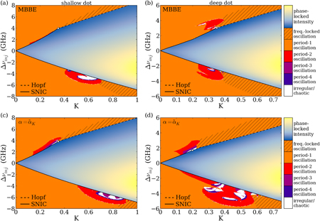
Figure 3. Two-parameter bifurcation diagrams of an optically injected (a), (c) shallow-dot and (b), (d) deep-dot QD laser. The color code denotes the number of intensity extrema found at each (K,Δνinj) parameter point, using the MBBE model (a), (b) and the MBBE with an α-factor (c), (d), respectively. The solutions were obtained numerically by sweeping the injection detuning outwards from Δνinj = 0. The light-blue to light-yellow shaded region shows the increasing laser intensity in the phase-locked region, where the QD laser emits cw light. The other color code denotes periodic oscillations (orange to dark blue), as well as chaotic or quasi-periodic behavior (white). The hatched region denotes phase-bounded oscillation, where the mean output frequency is equal to νinj. The solid and dashed lines denote SNIC and Hopf bifurcation lines, respectively, delimiting the phase-locked region. J = 2Jth.
Download figure:
Standard image High-resolution imageThe bifurcation diagrams in figure 3 were obtained by using the independent refractive-index-gain dynamics (top), or an α-factor (bottom). The type of solution is indicated by the color code. The light-blue to light-yellow shaded region denotes parameter values for which a steady-state is reached, with the color indicating the relative laser intensity, increasing from blue to yellow. This region corresponds to the locking tongue, where the QD laser is phase-locked to the injected optical signal (cf [6], where locking tongues are discussed for a simplified QD laser model). Upon leaving this locking tongue, the cw solution is lost either in a saddle-node on an invariant cycle (SNIC) bifurcation, shown by the continuous black line, or in a Hopf bifurcation (dashed black line), and both coalesce in a zero-Hopf point (open circle). The QD laser then begins to operate in an oscillatory regime, which in the simplest case is a period-1 oscillation (running phase solution, orange shaded). For larger values of the injection strength, these periodic solutions can be phase-bounded (hatched area). Here, the electric field follows a limit cycle, however, its average phase velocity is zero, such that the laser is on average still locked to the frequency of the injected field [55–58].
Close to the zero-Hopf points, where the SNIC and Hopf bifurcation lines meet, parameter regions of complex dynamics outside of the locking region exist, denoted by a different color code (red to dark blue), corresponding to periodic orbits of higher periodicity. These orbits are created in period-doubling bifurcations, which can be embedded within each other, leading to a period-doubling cascade and a subsequent birth of a chaotic attractor [49]. The regions of chaotic and quasi-periodic dynamics are depicted as white areas.
When comparing the numerical results of the MBBE model with that using an  , the shape and extent of the phase-locked parameter region shows a very good agreement for both models. The dynamics outside of the locking tongue, however, shows large differences. For the shallow dot structure, the use of
  leads to a complicated bifurcation structure for K around 0.25 for positive Δνinj. In the MBBE model, this region is confined to a very narrow area outside of the SNIC bifurcation line. For negative detuning, the period-doubling bifurcation regime shifts toward lower K and is also reduced in size, however retaining its general shape.
The differences for the deep QD laser are even stronger. The overall bifurcation scenario is comparable to the shallow dot case when using constant  , with a slightly larger region of complex dynamics due to a weaker damping of the ROs in the deep dot laser [6]. The MBBE model, however, predicts a vastly different scenario. Here, the extension of the bifurcation structures outside of the locking tongue is much smaller, with only very small islands of complex dynamics embedded in the areas of period-2 oscillation.
In order to verify the predictions of our balance equation model, we compare its numerical results with one-dimensional bifurcation diagrams of the shallow dot laser calculated using the microscopic model (see appendix A) for constant K in figure 4, corresponding to a vertical slice through the bifurcation diagrams in figure 3. The bifurcation diagrams reveal a very good quantitative agreement between the MBBE and microscopic models for both the shallow and deep dots (not shown here). Note, however, the slightly different value of K and scaling of the Δνinj-axis in figure 4(a), revealing slight differences in the position of the occurring bifurcations in the parameter space when using the MBBE model. These differences can be related to the different treatment of the scattering processes in the microscopic model, where an effective relaxation rate approximation is used, whereas the MBBE model utilizes microscopically calculated Boltzmann-like scattering terms. Nevertheless, the comparison shows that our simplified balance equation system can very well reproduce the results of the microscopic model. The comparison with the  model, as seen before, shows strong qualitative differences. While around K ≈ 0.70 the bifurcation structure outside the phase-locked region shows some similarities to that observed for the MBBE and microscopic models in figure 4, no value of K was found at which the
  model could reproduce these dynamics as closely as the MBBE model.

Figure 4. One-dimensional bifurcation diagrams of the shallow dot laser under optical injection for (a) the microscopic model, (b) the MBBE model and (c) the MBBE model with constant  . Shown are the extrema of the laser intensity obtained for different values of Δνinj. Note the slightly different value of K and scaling of the Δνinj-axis in (a).
Download figure:
Standard image High-resolution imageThe observed differences in the two descriptions of the refractive index dynamics can be understood by investigating the transient evolution of the optical susceptibility. In figure 5 we plot the dynamics of χ of the optically injected shallow dot laser (K = 0.5) upon instantaneous switching of the detuning of the injected signal from 0 GHz (resonant) to a finite value. As long as the detuning is not too large, i.e. still within the locking tongue, the laser reaches a steady-state. The steady-state susceptibility χs then lies on the black curve in figure 5, which shows a near-linear relationship between real and imaginary part of χ. Such a linear relationship can very well be approximated by an α-factor, which explains the good agreement in the shape of the locking tongue between both models. However, looking at the transient evolution of χ(t) upon switching of Δνinj (blue solid curves) and the periodic oscillation when choosing Δνinj outside of the locking range (green dashed line), it becomes obvious that the dynamic transients cannot be described by such linear relationship, as χ(t) can exhibit complicated dynamics itself. Especially when discussing dynamically complex solutions where the electric field exhibits dynamics on the timescale of the carrier lifetimes, the charge carrier distribution is no longer able to adiabatically follow the electric field dynamics. Using an α-factor would restrict Reχ to a functional dependence on Im χ and thus artificially constrain the dynamics of χ(t) in phase-space. Thus, models with the α-factor cannot reproduce the QD laser dynamics which we observe by using the MBBE model described above.
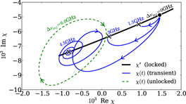
Figure 5. Transients of the optically injected QD laser in the complex susceptibility plane (Reχ,Im χ) for shallow QDs. The thick black line marks the steady-state values χs of the susceptibility for K = 0.5, and Δνinj varied across the phase-locked detuning range. The susceptibility at Δνinj = 0 GHz is marked by the black circle, and the black crosses mark χs at detuning values of (from right to left) 1.5, 3, 4.5 GHz, respectively. The blue lines show the transient evolution of χ after instantaneous switching of the injection detuning from Δνinj = 0GHz to 1.5, 3.0 and 4.5 GHz, respectively. The dashed green line marks the transient of χ for Δνinj = 6 GHz, for which the laser is unlocked and exhibits periodic intensity oscillations.
Download figure:
Standard image High-resolution imageFor the deep dot laser, the bifurcations outside of the locking tongue are, surprisingly, nearly symmetrical in Δνinj, which would generally only be expected for α = 0 in conventional models, i.e. for no index variation at all. This can be explained by the comparably long scattering lifetimes for the deep dots, leading to a very slow coupling between the resonant GS states and the off-resonant states. The dynamics of the electric field inside the QD laser with deep QDs are now much faster than the carrier dynamics, such that the carrier-induced index variation is unable to follow the dynamics and shows only very little variation. This is illustrated in figure 6, where the time series of the QD GS and ES occupation for an oscillatory parameter combination are shown (subgroup averaged), revealing similar changes in the GS occupation between deep and shallow dot, but much smaller variation of the ES occupation in the deep dot. Thus, in the limit of very slow charge carrier exchange, the QD laser dynamics outside of the locking tongue approach what would be expected for α = 0, whereas the phase-locking boundaries are similar to those predicted from a finite α > 0.
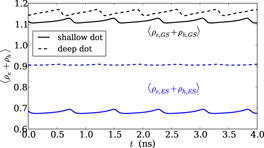
Figure 6. Time series of the sum of the mean electron and hole occupation in the QD GS (black) and ES (blue curves), averaged over the subgroups, for K = 0.2 and Δνinj = 2 GHz, both for the shallow (solid) and deep dot (dashed), using the MBBE model. J = 2Jth.
Download figure:
Standard image High-resolution imageFigure 7 illustrates this interpretation by comparing results for the full MBBE model with results obtained with α = 0. The bifurcation structure of the deep QD laser outside of the locking tongue closely resembles that predicted from using α = 0. Thus, the dynamics of the deep QD laser can be closely approximated by two different α-factors: on the one hand, the steady-state solutions and their stability can be rather well described by using the adiabatic  as defined in equation (B.3). On the other hand for oscillatory and complex solutions, the slow charge carrier exchange leads to a weak influence of the resonant carrier dynamics on the off-resonant states, and thus the dynamics closely resemble those of an device with α = 0. This approximation, however, is only valid for QDs that are very weakly coupled to the off-resonant charge carrier reservoir. In the shallow dot case the situation is different. It is still possible to define an adiabatic
  -factor to describe steady-state solutions, however, the coupling of resonant and off-resonant states can lead to a strong nonequilibrium when dynamic solutions emerge. In that case, no α-factor can be defined to describe the QD laser dynamics.
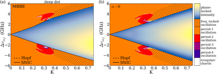
Figure 7. Two-parameter bifurcation diagrams of the optically injected deep-dot QD laser, cf figure 3. (a) MBBE model and (b) MBBE with α = 0.
Download figure:
Standard image High-resolution image3.2. Delayed optical feedback
Another much studied experimental configuration leading to complex dynamics is a semiconductor laser with time-delayed optical feedback. The dynamics induced by the optical feedback are of major importance for applications of semiconductor lasers, since it can lead to an unwanted deterioration of the laser performance [59, 60], and on the other hand can be utilized, e.g. for chaos communication [61, 62] or random number generation [63, 64].
Time-delayed feedback is modeled by using equation (30). We choose τec = 100 ps, corresponding to a feedback length of ℓ = 15 mm. In this short external cavity regime, characterized by a feedback length much smaller than the inverse RO frequency, τec ≪ (fRO)−1, the response of the QD laser to the time-delayed feedback sensitively depends both on the feedback strength Kfb as well as the feedback phase C [16, 46, 65]. To obtain a complete analysis of the bifurcation scenario, we again numerically calculate two-parameter bifurcation diagrams, now in the (Kfb,C) parameter space, by sweeping the feedback phase for each given Kfb upwards. As before, we compare the MBBE model with feedback, equation (30), with a model using α similar to equation (31), which reads

We again use  evaluated at K = 0 for the calculations with α, as it should describe the QD laser reacting to an optical perturbation in the best way possible.
When optical feedback is introduced in QD lasers, new steady-state solutions which are referred to as external cavity modes (ECMs) are born. ECMs describe the steady-state solutions corresponding to standing wave modes of the coupled laser and external cavity system [66–68]. The electric field then follows the relation

where Es is a constant field amplitude. The constant frequency shift compared to the free-running laser is given by  , where ωs denotes the frequency of the ECM. The number of existing ECMs depends on the delay time τec and the amplitude-phase coupling, where both a higher delay and a stronger amplitude-phase coupling leads to a higher number of possible ECMs fulfilling the standing wave condition. Due to the existence of multiple ECMs, the laser with feedback often exhibits multi-stability as well as complex and chaotic dynamics when the stability of a given ECM is lost [12, 15].
We simulate the balance equation model using either equation (30) or (32) for the comparison of both QD laser models with optical feedback. The resulting bifurcation diagrams are shown in figure 8. In figures 8(a) and (c) the faster scattering rates (shallow dot) lead to a stronger damping of the laser ROs, which in turn simplify the existing bifurcation scenarios, which was extensively studied in [16]. The slower scattering rates of the deep dot structure, on the other hand, lead to more complex bifurcation structure as shown in figures 8(b) and (d). In both cases, however, the use of an α-factor leads to a larger region of complex and oscillatory dynamics when compared to the full MBBE model equations. In the shallow dot case, the model predicts only a very narrow region of complex dynamics where the first ECM loses its stability, and a different ECM is reached afterwards, evident from the sudden change in intensity. More importantly, the critical feedback strength, for which non-cw dynamics appear, is predicted to be higher in the full MBBE model compared to what the α-factor model predicts. This suggests that the experimentally observed low sensitivity of QD lasers to optical feedback is, in fact, not only caused by the stronger damping of ROs and a low α-factor, but also by the independent dynamics of the real and imaginary part of the gain.
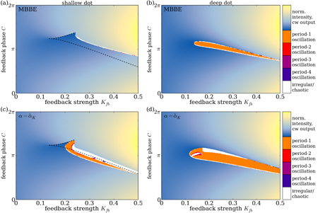
Figure 8. Two-parameter bifurcation diagrams of the (a) shallow-dot and (b) deep-dot QD laser with optical feedback, using the full MBBE model (top) and an α-factor (bottom), respectively. The color code (orange to white) shows the number of extrema found at each parameter point, and the color shading (light-blue to light-yellow) shows the increasing intensity of the laser when cw-output is emitted, cf figure 3. The dashed lines show the approximate position of the saddle-node bifurcation lines, which meet in a cusp point. In the deep dot case the saddle-node lines lie within or close to the regions of oscillatory dynamics and are thus not accessible by direct integration. J = 2Jth.
Download figure:
Standard image High-resolution image4. Conclusion
In summary, we presented an energy balance and carrier density rate equation model for QD lasers that is derived from a microscopic theory. The MBBE model takes into account carrier heating and describes the index change due to carriers in off-resonant states rigorously, without the use of an α-factor. Equally important, it is applicable to numerical bifurcation analyses of QD lasers subjected to either external optical injection or time-delayed optical feedback.
We have investigated the differences in the dynamics of QD laser structures arising from using an α-factor, compared to the dynamics predicted from the model with dynamic gain and index changes. Depending on the timescale of the charge carrier scattering, we have observed different kinds of dynamic behavior of the QD laser. In the limit of very slow carrier scattering, e.g. as encountered for QDs with very large localization energies, the index change becomes increasingly smaller and the dynamic scenarios resemble those predicted by choosing α = 0, while adiabatic index changes between steady states can still be described by a finite, adiabatic  . For shallow QDs with faster charge carrier scattering, the laser dynamics are appreciably influenced by the independent index dynamics. Thus no α-factor can be defined which would predict the observed dynamics.
In general we have found that the bifurcation structure and dynamics of the QD laser system described by the energy balance equations is much simpler than what is predicted from models employing an α-factor. In the short external cavity regime of feedback setups, the full energy balance model equations predict a higher critical optical feedback strength than the rate equation models using an α-factor. Thus, we conclude that the higher tolerance of QD lasers to optical perturbations and the observed simpler dynamics is not only caused by the strongly damped ROs commonly found in QD lasers, but to a large degree by the additional degree of freedom introduced by the independent dynamics of the gain and index changes.
Acknowledgments
This work was supported by DFG within SFB 787, the US Department of Energy's National Nuclear Security Administration under contract no. DE-ACD4-94AL85000, and Sandia's Solid-State Lighting Science Center, an Energy Frontier Research Center (EFRC) funded by the US Department of Energy, Office of Science, Office of Basic Energy Sciences.
Appendix A.: Microscopic model
The microscopic description of semiconductor QD laser devices can be done on varying levels of complexity. Here, we apply a model derived from semi-classical laser theory, which treats charge carrier collisions at the level of effective relaxation rates.
In the microscopic model the electric field is driven by the dynamics of the microscopic polarization of each QD subgroup:


The QW charge carrier distribution is described by tracking the occupation probability of individual k2D states in time, allowing the description of nonequilibrium distributions. Additionally, the k3D-resolved occupation of bulk states are taken into account. The dynamic equations for these charge carrier states are then given by
along with the scattering expression for the QD occupation probabilities

where  describes the relaxation between QD states as given in equation (11). The scattering here is described within the relaxation rate approximation, leading to the relaxation of the given carrier occupations toward a common quasi-Fermi distribution. These distributions are calculated from carrier number and energy conservation conditions, e.g. for determining (μ(QW,GS)b,T(QW,GS)b), one needs to solve
and analogous conditions for all other scattering processes. Carrier–carrier scattering in general will lead to an increase in carrier temperature, while we additionally assume carrier–phonon scattering between QW and bulk states, which cools the distribution down to the lattice temperature. As such, only the quasi-Fermi levels μ(QW,bulk)b,c–p are unknown, and solving only equation (A.6) is sufficient for the carrier–phonon scattering. We incorporate carrier–carrier Auger scattering (rate γc–c = 1 ps−1) and carrier–phonon scattering (γc–p = 0.1 ps−1) between QW and bulk states (superscript (QW,bulk)), QW and QD states ((QW,GS) and (QW,ES), Auger only), with their Auger-scattering rate given by τb,m−1 = (Sin,capb,m + Sout,capb,m), as well as thermalization of QW electron and hole distributions ((QW,th), γth = 1 ps−1) toward the temperature of the respective opposite charge carrier species b'. The effective loss terms are given by

with n3D the bulk carrier density per unit area. The electrical pumping is described in equation (A.4) by the pump rate γJ = 1 ps−1, and the pump carrier distribution f(εb(k3D),μJb,Tℓ), with its quasi-Fermi level determined from the condition

The above equations together with equations (5) and (8) then form the microscopic QD model.
An inclusion of many-body effects within the Hartree–Fock approximation could be done in a straightforward way [23, 26], leading to a dynamic renormalization of the single-particle energies and the Rabi frequency. We have not included these effects in the present work in order to highlight the differences in the dynamics arising from the independent dynamics of the carrier-induced gain and index changes.
Appendix B.: Failure of characterizing quantum-dot lasers by an α-factor
We evaluate the phase dynamics of the electric field. The phase-response of semiconductor lasers, i.e. the coupling between amplitude and phase of the electric field, is commonly modeled by introducing the so called linewidth enhancement factor α [22, 69]. It is then assumed that there exists a linear relationship between carrier-induced changes in the gain and refractive index. Expressed in terms of the optical susceptibility χ(ω) = 2εbg/(iωΓ)g(ω), α is defined as

where ∂/∂N is the derivative with respect to the total charge carrier number N, containing all carriers inside the QD subgroups and the reservoir. The exact variation ∂N must be determined from the system dynamics. Due to the intricate scattering dynamics between the resonant and off-resonant carrier states in QD devices, the carrier variation depends on the exact change of operating conditions, which can lead to strongly different α-factors for different types of applications [24], which explains the vast range of values for α in QD lasers reported in the literature [70–74]. In order to illustrate this difference, we evaluate the response of the laser device to changes of the pump current below threshold:

where χs(ω)|J denotes the steady-state susceptibility at the pump current J. The tilde here denotes the evaluation of the difference of the steady-state susceptibilities, after all transients have worn off. We thus define  as the adiabatic α-factor of the system. The
  evaluated in this way corresponds to measurements that evaluate amplified spontaneous emission spectra below threshold [75] in order to yield an α-factor. Above threshold, the before-mentioned method cannot be applied due to the clamping of the steady-state gain at the threshold value. We therefore need to apply a different method above threshold. Using either the optical injection or feedback setup we evaluate

defined similarly to equation (B.2), but instead of changing the pump current, a weak resonant (Δνinj = 0) optical signal injected into the cavity is considered, and either the injection strength K or the feedback strength Kfb is varied. This optical signal induces a change of the electric field inside the cavity, which in turn varies the carrier distribution by stimulated emission, leading to gain and index changes.
The two methods to determine an α-factor are numerically evaluated for both types of QDs and shown as a function of the pump current in figure B.1. Below threshold both QD structures show an increase of the adiabatic  -factor below threshold, in agreement with experimental findings [76]. For the shallow dots
  reaches values around 1.5 at threshold, while the deep dot case exhibits values up to 1.0. This difference can be explained by the larger energetic distance of the resonant QD transitions and the off-resonant continuum transitions in the deep dot case, as it reduces the impact of the reservoir carriers on the index change at the optical transitions.

Figure B.1. Calculated adiabatic  -factor
  as a function of the pump current J in units of the threshold current Jth, for shallow (blue diamonds) and deep (red circles) QDs. Below the threshold current, marked by the vertical dashed line, the change of the steady-state susceptibility under increasing pump current Δχs|J is evaluated (equation (B.2)), whereas for J > Jth, the change Δχs|K is induced by slightly increasing the injection strength from K = 0 to 0.01 for Δνinj = 0 GHz (cf equation (B.3)).
Download figure:
Standard image High-resolution imageAbove threshold,  , defined in equation (B.3), is evaluated for both laser systems. It is immediately visible that the definition of
  , which considers the change of χS by an optical signal, leads to drastically different values than the method based on the gain and index change under pump current variation. This difference can be traced to different changes in the charge carrier occupation when evaluating
  and
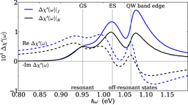
and  . In figure B.2, the differential changes in the steady-state susceptibility Δχs under changes of the pump current (black curves) and changes in the injection strength (blue curves) are shown. From the changes of Im Δχs (solid lines), it can be seen that changes in the pump current lead to a larger variation of the occupation of off-resonant states when compared to the changes under the influence of an optical signal. This then leads to a stronger relative change in refractive index, proportional to Re Δχs (dashed lines) at the optical transition. This in turn leads to a larger value of
  .
.
Figure B.2. Changes in the steady-state gain spectrum χs(ω) of the shallow-dot QD laser upon increasing the pump current from 0.99Jth to Jth (black curves), and upon switching the injection strength between K = 0.02 and 0 at J = 1.01Jth (blue curves). The solid and dashed lines show changes in the imaginary and real part of the steady-state susceptibility, respectively. The vertical lines denote, from left to right, the respective transition energies of the QD GS, QD ES and QW band edge.
Download figure:
Standard image High-resolution image
The different values of  and
and  illustrate the difficulty of characterizing QD laser devices by using an α-factor. The laser can react vastly differently under different perturbations even at the same operational point.