Experimental determination of droplet collision rates in turbulence

R Bordás; Ch Roloff; D Thévenin; R A Shaw

doi:10.1088/1367-2630/15/4/045010

1. Introduction

Turbulent flows containing small, dispersed particles are encountered in numerous technical and environmental systems. For instance, rain precipitation processes in atmospheric clouds are influenced by the interaction of a dispersed liquid phase with the turbulent properties of the gaseous phase [1]. Clouds are of special relevance today because of the important part they play in climate science. The large-scale processes controlling climate and weather can only be described with sufficient accuracy when small-scale processes are fully understood. One of the most important issues at small scale is turbulence-modulated particle clustering and collision. Many theoretical studies have been devoted to this topic but comparison with experimental work would improve physical understanding and help identify the most reliable models to date. Hence, the present work is focused on that aspect: can current theoretical expressions for the collision rate of particles in turbulence and under the influence of gravity, account quantitatively for measured collision rates in a controlled laboratory experiment? This work is an extension of [2], in which a single measurement technique has been employed for a slightly different configuration and compared with classical theoretical correlations. The results have revealed noticeable differences between measurements and theory. In an effort to check and generalize these findings, a second, independent measurement technique and additional, more advanced correlations are now considered.

Careful theoretical work on collision rates of small, heavy particles in turbulence, with relevance to atmospheric clouds, already began in the 1950s with Saffman and Turner [3]. In the past decade, important new theoretical advances, driven largely by numerical simulations of turbulence, have been documented (e.g. [4–7]). For a recent review on this topic see also [1]. The theory has advanced to the point where quantitative predictions for the collision rate of droplets settling through turbulent air are now possible, over the whole droplet size range and turbulence conditions relevant to clouds. In order to allow direct comparisons with theory, the objective of this work is to provide a direct experimental measure of the collision rates for a known, polydisperse population of droplets in a well-characterized and reproducible turbulent flow. The droplet and turbulence properties are measured independently but completely. Controlled laboratory experiments are an attractive complement to measurements in atmospheric clouds (either mountain-based or airborne) since in the latter case the real environment is unsteady, non-reproducible, and some relevant boundary or initial conditions cannot be determined. In contrast, all relevant conditions are controlled, reproducible and measurable using a wind tunnel experiment, allowing long-time averaging since turbulence and particle properties are statistically stationary [8]. Such averaging is absolutely crucial here because collisions are indeed rare events, especially for the largest, least numerous drops [9]. As a consequence, statistically relevant statements are only possible when acquiring experimental data over very long times.

The problem of particle collisions in turbulence is extremely complex. Only a few measurements are available to validate and guide theory as yet. One main approach has been to consider only specific subsets underlying collision theories, usually divided into (i) transport effects, e.g. changes in particle relative velocity resulting from turbulent acceleration, (ii) spatial clustering of particles due to mixing and inertia, and (iii) hydrodynamic interactions of particles in close proximity. Particle clustering has been investigated particularly intensely [10–16]. The direct experimental determination of relative velocity has also been discussed in the literature [17]. However, measuring collision efficiency remains extremely challenging. Very few studies have been focused on direct measurements of the collision rate itself, and those have usually been carried out under conditions where gravity does not play a significant role (e.g. [18]). The present work should therefore be useful to complement previous studies, delivering experimental data for evaluating existing theories and guiding future theoretical efforts.

The paper is organized as follows. In section 2 theoretical expressions are provided for collisions of small particles in turbulent flows, taking into account the influence of gravity. The emphasis is set on expressions that can be compared quantitatively with the measurements. Section 3 describes the experimental setup and section 4 provides experiment and analysis details relevant to the particle tracking problem, necessary for deriving collision rates from those measurements. All results, including the turbulence and particle size characterization, evaluation of the collision detection and calculation of the total collision rate, are given in section 5. At the end of that section the measured collision rates are compared to the theoretical expressions from section 2. Finally, the results and their implications for theory, as well as a summary of conclusions, are given in section 6.

2. Collision theories and models

The average collision rate per unit volume for droplets of radii r₁ and r₂ is proportional to the respective particle number densities n₁ and n₂, and to the collision kernel Γ₁₂ that accounts for both the effective collision cross section and for the rate at which droplets of radius r₁ encounter those of radius r₂: $\dot {N}=n_1 n_2 \Gamma _{12}$ . The collision kernel has its roots in gas kinetic theory, and in quite general terms it can be expressed as [19–21]

$\begin{equation} \Gamma_{12}=2\pi R^2 w_{\mathrm{r}} g_{12} E_{12}, \end{equation} \tag{ 1 }$

where 2πR² is the geometric collision cross section, in which R = r₁ + r₂ is defined as the collision length, w_r accounts for the particle relative velocity and g₁₂ is the radial distribution function that accounts for the presence of spatial correlations at the collision length. The term E₁₂ is the collision efficiency that results from hydrodynamic interactions between droplets near collision, and therefore can be thought of as giving the effective cross section when multiplied by 2πR². Coalescence efficiency is sometimes defined, allowing for the possibility of droplet collision followed by bounce, but that is thought to be close to unity for droplets smaller than several hundred micrometers in radius [22]. Such a coalescence efficiency will therefore not be considered in what follows, concentrating on the smaller droplets relevant for rain initiation. In this section different expressions from various authors are presented, taking into account the different contributions to the collision rate. This is meant to be only an overview and not a comprehensive review, focusing on the expressions relevant for cloud droplet collisions and directly comparable with the measurements described later in sections 3 and 4.

The simplest contribution to the relative velocity results from the different terminal fall speeds of droplets with different sizes. In the Stokes limit, droplets experience an exponential relaxation to their terminal fall speed v_p = τ_pg, where τ_p is the inertial response time and g is the gravitational acceleration. In most atmospheric clouds and in the laboratory experiments considered here, the droplets are embedded in a turbulent flow and the challenge is therefore to identify and quantify the various contributions of turbulence to the relative velocity. The most direct approach, due to Abrahamson [23], assume that droplets are decoupled from the flow, i.e. strongly inertial, and that the fluid velocity variance directly quantifies the droplet relative velocity

$\begin{equation} w_{\mathrm{r}}= 2\left(\frac{2}{\pi}\right)^{1/2}\left[v'^{(1)}+v'^{(2)}\right]^{1/2}. \end{equation} \tag{ 2 }$

The combined relative velocity arising from turbulence and gravity can be expressed empirically if the components of the velocity variance v'⁽ⁱ⁾ can be measured directly.

A theoretical approach that allows droplet relative velocity to be determined directly from the turbulence properties is much more powerful, and several such expressions are considered in what follows. In all cases, the influence of turbulence is considered in the limit of particle size smaller than the turbulent energy dissipation length and for particle density greater than fluid density, both of which are reasonable assumptions for cloud droplets in air. The classic expression for droplet relative velocity resulting from turbulence and gravity, obtained by Saffman and Turner [3], is

$\begin{equation} w_{\mathrm{r}} = \left(\frac{8}{3\pi}\right)^{1/2}\left[ \frac{1}{3}R^2\frac{\varepsilon}{\nu} + 2(\tau_{p2}-\tau_{p1})^2\left\langle\left(\frac{\mathrm{D}u}{\mathrm{D}t}\right)^2\right\rangle + (v_{p2}-v_{p1})^2 \right]^{1/2}. \end{equation} \tag{ 3 }$

Contributions from turbulence include the relative velocity induced by fluid velocity shear and by fluid Lagrangian accelerations, in the first two terms on the right-hand side, respectively. The last term on the right-hand side is the difference in terminal fall speeds.

Dodin and Elperin [4] showed that the Saffman–Turner expression, while appropriate in its basic features, does not reach certain limits correctly (e.g. zero inertia). They thus decomposed the relative velocity into turbulent and gravity-induced components and assumed that the turbulent component is normally distributed to obtain

$\begin{equation} w_{\mathrm{r}}= 2\left(\frac{2}{\pi}\right)^{1/2}\sigma f(b), \end{equation} \tag{ 4 }$

where

$\begin{equation} \sigma^2=\frac{1}{15}R^2\frac{\varepsilon}{\nu}+(\tau_{p2}-\tau_{p1})^2\left\langle\left(\frac{\mathrm{D}u}{\mathrm{D}t}\right)^2\right\rangle, \end{equation} \tag{ 5 }$

with

$\begin{equation} b=\frac{g|\tau_{p2}-\tau_{p1}|}{\sigma\sqrt{2}} \end{equation} \tag{ 6 }$

and

$\begin{equation} f(b)=0.5\sqrt{\pi}\left(b+\frac{0.5}{b}\right)\textrm{erf}(b)+0.5\exp(-b^2). \end{equation} \tag{ 7 }$

This equation reduces to the proper limits and has the advantage of being relatively straightforward to implement. The expressions of Abrahamson, Saffman–Turner, and Dodin–Elperin account for what is sometimes referred to as the turbulent transport contribution to the collision rate. However, they do not include any spatial correlation or collision efficiency.

Ayala et al [6] proposed an integrated parameterization of the turbulent collision kernel that takes into account both the turbulent transport and the accumulation (or spatial correlation). In order to simplify the implementation of the transport term, they derived an approximate form

$\begin{equation} w_{\mathrm{r}}= \sqrt{\frac{2}{\pi}} \left(\sigma^2 + \frac{\pi}{8} (\tau_{p1} - \tau_{p2})^2 |g|^2 \right)^{1/2}. \end{equation} \tag{ 8 }$

The approximation leads to a maximum overestimation of 2.5% compared to the exact equation [6], which is negligible compared to the experimental uncertainties discussed in this paper. Equation (8) includes separate contributions of gravity and turbulent transport. The turbulent term contains horizontal and vertical droplet velocity components, as well as their cross-correlation:

$\begin{equation} \sigma^2 = \left\langle\left(v'^{(1)}\right)^2\right\rangle + \left\langle\left(v'^{(2)}\right)^2\right\rangle - 2\left\langle\left(v'^{(1)}v'^{(2)}\right)\right\rangle. \end{equation} \tag{ 9 }$

The corresponding expressions for the velocity components are quite complex and can be found in the original reference (pp 37–8 in [6]). It should be noted that these terms depend on the relative importance of gravitational settling. The accumulation, expressed through the radial distribution function, follows the form suggested by Chun et al [5]:

$\begin{equation} g_{12}(R)=\left(\frac{\eta^2+r_c^2}{R^2+r_c^2}\right)^{C_1/2}, \end{equation} \tag{ 10 }$

where

$\begin{equation} \left(\frac{r_c}{\eta}\right)^2 = |St_2 - St_1| F, \end{equation}\noindent \tag{ 11 }$

where St is the droplet Stokes number and C₁ and F are functions of the gravitational and turbulent accelerations (pp 38–9 in [6]). We note from equation (8) that when turbulent transport and accumulation vanish, i.e. σ² = 0 and g₁₂ = 1, the expression reduces to the expected w_r∝(τ_p1 − τ_p2)|g| for pure gravitational sedimentation.

Lastly, the combined influence of gravity and turbulence on droplet collision rates has been thoroughly studied in a series of papers by Pinsky et al [7, 24–27]. The results of the work are summarized in tabular form in [7] for three different turbulent kinetic energy dissipation rates and for droplet radii between 1 and 21 μm (see their tables A4–A6, in which the kernels are normalized by that for gravitational sedimentation). For droplets with radii greater than 21 μm it is assumed that the droplet relative velocity is dominated by gravitational sedimentation alone. Furthermore, the accumulation or clustering effect can be included by multiplying the kernel with the empirical expression [28]

$\begin{equation} P_{\mathrm{clust}} = 1 + 0.333 (St_1 \,St_2)^{0.317}. \end{equation} \tag{ 12 }$

The collision efficiency is considered the most uncertain aspect of collision rate theories, even if some conclusions have emerged from recent work [1]:

collision efficiency in a turbulent flow is a random number with a mean value that is typically larger than the gravitational collision efficiency;
the collision efficiency increases most strongly as d₂/d₁ → 1;
the results depend sensitively on the size of the larger droplet from a colliding droplet pair;
when the effect of turbulence on collision efficiency is also considered, the warm rain initiation time could be reduced up to a factor of two [29].

Finally, the collision efficiency is a critical issue for comparing measured collision rates with any collision theory. In this work we consider collision efficiencies that are derived from the work of Pinsky et al [7, 24, 27] (see tables A1–A3 in [7]) and from Wang et al [29–31] (see table 1 in [29]) for several different turbulent kinetic energy dissipation rates. For purely gravitational settling the collision efficiencies from Hall [32] are considered.

3. Experimental setup

3.1. Two-phase wind tunnel and droplet injection

A wind tunnel available at the Laboratory of Fluid Dynamics and Technical Flows has been used for the present experimental investigation of dispersed two-phase flows under conditions approximately corresponding to those found in cumulus clouds [2]. This wind tunnel can be used to investigate a variety of two-phase (air/liquid) flows. It is a fully computer-controlled, Prandtl or Göttingen-type wind tunnel, shown in figure 1 (left). Operation with a closed test section enables the controlled and reproducible investigation of two-phase mixtures in the measurement section, with dimensions H × W × L = 500 × 600 × 1500 mm³ and with optically transparent side and top windows in the visible spectrum. In this manner non-intrusive measurements are possible, which is essential for high-quality experimental investigations of such flows.

Figure 1. Refer to the following caption and surrounding text. — **Figure 1.** Göttingen-type two-phase wind tunnel with closed test section (left). Measurement section with employed coordinate system, double spray injection head, passive grid for turbulence homogenization, horizontal cylindrical bluff-body for local turbulence modifications, and also vertical measurement plane (x = 0 mm) in red (right).
Download figure:
Standard image

The air flow velocity can be continuously controlled from 0.3 to over 50 m s⁻¹ with a resolution of 0.03 m s⁻¹, limited by the electronic regulation. Turbulence intensity of the undisturbed air flow in the measurement section is below 0.5%. Nevertheless, the droplet injection, sketched on the left part of figure 1 (right), increases the velocity fluctuations and thus the turbulence intensity (up to 15% depending on the configuration).

The dispersed phase was added to the air flow with the help of an injection system. The droplet injection nozzle has always been installed upstream of the test section. It is connected to a pipe with an 18 mm outer diameter mounted on the upper wall of the tunnel. In order to reduce the influence of the injection system (wake of the profiled injector support), an airfoil was mounted on the nozzle, and the nozzle was fixed 630 mm upstream of position x = 0 (inlet of the optically accessible measurement section and vertical measurement plane). The sprays were actuated by means of eccentric screw pumps. The number of revolutions per minute (rpm) was set with the help of a frequency regulator to a prescribed value by means of a proportional–integral–derivative (PID) control algorithm coded in LabView®, regulated according to the measured water volume flow rate before the spray injection. In this manner it is possible to obtain a steady water volume flow rate, through which the droplet diameter remains constant over a long period of time. This is needed since measurements are operated under constant conditions over many hours to gather statistically significant data.

In order to investigate rain formation and cloud droplet interactions, full cone pneumatic atomizing nozzles were used (types 166.208.16.12 and 154.104.16.14 from the company Lechler GmbH, Germany), relying on the liquid pressure principle and applying an air gauge pressure of 1.2 bar [33]. The system can be employed with either one single or two injection heads simultaneously, the latter being sketched in figure 1 (right). Therefore, not only monomodal but also strongly bimodal droplet size distributions can interact within the test section. For rain initiation and cloud droplet interactions, two-fluid atomizers (small droplets) are employed. The selected nozzles deliver a typical six-hole spray pattern because of the six orifices in the nozzle, each with a diameter of 1 mm. Injecting the water droplets in the counter-flow direction, the droplets become more homogeneously distributed as they travel downstream and the six-hole pattern is strongly weakened at the entrance of the measurement section. Since most of the disturbances caused by the support of the nozzle were in the upper half of the measurement section, only the lower half was finally measured. Different injection heads have been tested to create droplets with a narrow diameter distribution for each nozzle and leading to a plausible droplet size distribution (DSD) and droplet Stokes numbers for cumulus clouds experiencing drizzle formation (figure 2).

Figure 2. Refer to the following caption and surrounding text. — **Figure 2.** DSD for configurations M3 and M4 at two selected points of the entrance vertical plane in the measurement section (x = 0, y = 0, z = 0) and (x = 0, y = 150, z = 0), measured by PDA (left). Probability density functions of the droplet Stokes numbers for the selected positions (right). The Stokes numbers were calculated by equation (13).
Download figure:
Standard image

The coordinate system employed throughout the study is shown in figure 1 (right), with all measurements carried out in the present project at the entrance of the measurement section, defined as x = 0. All employed experimental techniques are non-intrusive and therefore without any consequence for the investigated flow. However, in order to measure the air properties, a small quantity of suitable tracer particles must be added to the flow. Such tracers follow the behavior of the continuous (air) phase much better than the considered droplets due to much smaller tracer Stokes numbers [34, 35], allowing in this manner an indirect measure of the gas flow properties. For this reason, the properties of both phases were finally measured in two separate steps:

1.
The velocity distribution and turbulence properties of the air phase were measured by means of laser-Doppler velocimetry (LDV). During these measurements in the continuous phase, the nozzle(s) was/were operating at the same pressure as in normal (spray) operation, but only with air and without water. Since the mass flow rate of air and water entering the nozzles are similar for normal operation conditions, typically $\dot {m}_{\mathrm {a}}/\dot {m}_{\mathrm {w}}=0.4$ , only minor flow changes should be induced by this necessary operation.
2.
All droplet properties including collision events are measured afterwards during normal operation, without adding any additional tracer particles.

Two different configurations are systematically employed for the later comparisons with theoretical predictions:

Configuration M3 is realized with a single droplet injection nozzle (type 166.208.16.12) and a cylindrical bluff body, but without passive grid. The cylinder, with a diameter of 20 mm, is located horizontally at the height of z = 90 mm, and at x = −150 mm perpendicular to the main flow direction (see figure 1, right). The shedding vortices should increase locally the velocity fluctuations and thus may increase the effect of preferential concentration [36]. In this manner an increased collision rate is expected in the wake of the cylinder. The resulting collision rates have been experimentally measured along a vertical z-profile (x = 0 and y = 0) behind the cylinder.
Configuration M4 contains both a passive turbulence grid and a bluff body. Additionally to configuration M3 a second atomizer with a different DSD was employed in a symmetrical configuration (both spray heads are installed at the height of z = 0 mm, y = −150 and +150 mm, respectively, as shown in figure 1, right). One atomizer was the same as in M3 and the additional one was a Lechler 154.104.16.14. Each nozzle had its own supply pump allowing an individual volume flow rate to be set and controlled. Besides the simultaneous application of grid and bluff body, the aim of this configuration was to create a broader droplet size distribution by means of two different nozzles (see figure 2) and thus impact noticeably resulting droplet collision events.

In what follows, all experimental measurement techniques and resulting properties are described.

3.2. Laser-Doppler velocimetry/phase-Doppler anemometry system for velocity and droplet diameter measurements

During this measurement campaign complementary non-intrusive optical measurement techniques were applied to determine the properties of both phases. A combined LDV/PDA (phase-Doppler anemometry) system was used to measure first the instantaneous velocity of the air (LDV) and afterwards to acquire the instantaneous velocity and simultaneously the diameter of the dispersed (droplet) phase (PDA). Further details can be found in [2].

3.2.1. Laser-Doppler velocimetry

LDV is a well-established technique that gives directly (without any calibration) information about flow velocity with high temporal resolution. Its non-intrusive principle and directional sensitivity make it very suitable for applications where sensors with physical contact are difficult or impossible to use. However, it requires tracer particles in the flow. Briefly described, LDV requires that two laser beams cross at their focal point. In the resulting measurement volume they interfere and generate a set of fringes. As tracer particles pass through these fringes, they scatter light into a photodetector. By measuring the frequency of the scattered light, the velocity of the tracer particles can be obtained, which is essentially identical to the flow velocity of the fluid for suitable tracer particles. In the present case, fog of polyethylene-glycol, PEG (ρ_PEG = 1130 kg m⁻³) is generated by a high volume liquid droplet seeding generator (Co. Dantec Dynamics, Denmark). The diameter range of the generated PEG droplets is 1–3 μm, with a mean diameter of 2 μm. The fog generator is able to deliver approximately 10¹³ particles s⁻¹, leading to a droplet number density of 10⁷ cm⁻³ and thus to a volume fraction of 4.65 × 10⁻⁵. Calculating the Stokes number St for tracer particles from their properties and using the Kolmogorov time scale τ_k, a maximum value of

$\begin{equation} St=\frac{1}{18}\frac{\rho_{\rm{par}}d^2}{\mu_{\rm{air}}\tau_{\rm{k}}}=0.02 \end{equation} \tag{ 13 }$

is found.

3.2.2. Phase-Doppler anemometry

PDA is an optical technique for measuring simultaneously the size and velocity of spherical particles, based on the same working principles as LDV. Note that, for all conditions in this project, the droplets are expected to be indeed spherical, as confirmed by shadowgraphy images (see later). The measurements are performed on single particles, thus allowing detailed analysis of particulate flows. The difference from LDV is in the receiving optics, which are placed at a well-chosen off-axis location. The scattered light is projected onto multiple detectors. Each detector converts the optical signal into a Doppler burst with a frequency linearly proportional to the particle velocity. The phase shift between the Doppler signals from different detectors is a direct measure of the particle diameter. Working principles of LDV/PDA can be found in detail in the literature [37]. Some adaption of the PDA-system was necessary to carry out the measurements in the flows considered in this work. In particular, laser beam power was set following recommendations found in [38, 39]. Note that PDA measurement in optically dense sprays are still highly challenging. Fortunately, the employed conditions in this project are still relatively far from such a regime.

A post-processing of the PDA measurements is necessary to obtain values for the number density or droplet concentration n [40, 41]. In the present work, the approach described in [42] was finally applied, improved by a factor η_vi allowing for correction of errors due to multiple particles occurring in the detection volume or to non-validation of particles, as proposed in [43].

The droplet-size-dependent calculation of the detection volume [43] was taken into account as well. Thus, the number density of the kth diameter class is finally obtained by

$\begin{equation} n_k=\frac{1}{T_{\mathrm{acq}}}\sum_{i=1}^{N_{\mathrm{sv}}} \frac{\eta_{\mathrm{vi}} t_{\mathrm{res},i}}{V_{\mathrm{det},k}}, \end{equation} \tag{ 14 }$

where T_acq is the acquisition time at a given measurement position, N_sv is the number of validated PDA-signals, η_vi is the correction factor described before, t_res,i is the residence time of the ith droplet and V_det,k is the size of the PDA detection volume of the kth diameter class. The PDA detection volume depends on the droplet size and is thus indirectly a function of the droplet velocity and of the burst duration in the detection volume.

The determination of the probability density function for the number density n_k(d_k) is a key property also for the later calculation of the collision rates. The corresponding post-processing allows the computation of both the probability density function of the droplet number density (n_k(d_k)) and its standard deviation (σ_n,k). The droplets are divided into size classes (d_k) with a given diameter resolution. The number density is computed separately for each size class using equation (14). In addition, the number density was calculated for different time scales by dividing the whole acquisition time T_acq into time intervals Δt. In this manner, the standard deviation σ_n,k can be calculated with

$\begin{equation} \sigma_{n,k}=\sqrt{\left(\frac{1}{T_{\mathrm{acq}}}\sum_{j=1}^{T_{\mathrm{acq}}/\Delta t}n_{k,j}^2 \Delta t\right)-n_k^2}. \end{equation} \tag{ 15 }$

This post-processing finally delivers the droplet concentration as a function of the droplet diameter, together with the corresponding standard deviation, as exemplified in figure 3 for two different positions in configurations M3 and M4.

Figure 3. Refer to the following caption and surrounding text. — **Figure 3.** Exemplary probability density functions of the experimentally determined droplet number density as a function of the size class, including the measured standard deviation as an error bar.
Download figure:
Standard image

3.3. Shadowgraphy system for detection of droplet collisions

Shadowgraphy imaging, applied here for the investigation of droplet–droplet interactions, is an imaging measurement method relying on a digital camera, an objective lens with high magnification, and background illumination lying on the same optical axis (see sketch in figure 4), as described for instance in [45]. As the droplets are illuminated from behind, their shadow image is recorded by the camera and the diameter of the droplets can be obtained with the help of a previously calibrated μm pixel⁻¹ value. Due to the dimensions of the wind tunnel test section, a far-field microscope (Questar QM1) is required for the present measurements, as already discussed in [44, 45]. The illumination has been provided by a water-cooled high power LED array consisting of 8 × 9 CREE XM-L T6 emitters. With the help of the triggered LED array a homogeneous and powerful background illumination was obtained. Operation in pulsed mode allowed even higher drive currents at short times, ensuring very high image intensities at short exposures. This is essential for acquiring reliably fast and small droplets. Using this shadowgraphy setup, two completely independent image evaluation methods have been applied in a post-processing step to detect droplet collisions. The main difference was in the magnification and in the method used to detect collisions:

Figure 4. Refer to the following caption and surrounding text. — **Figure 4.** Sketch of the optical shadowgraphy setup with (1) digital camera, (2) long distance microscope, (3) wind tunnel measurement section, (4) optical path of the imaging system, (5) diffuse LED illumination cone, (6) measurement volume and (7) water cooled LED array.
Download figure:
Standard image

1,
High magnification imaging using centricity indicators as detailed in [2]. This approach is simply called in what follows 'shadowgraphy'. For this technique the employed camera is an Imager Intense system with a 2/3'' CCD-sensor from LaVision (resolution: 1376 × 1040 pixel; pixel size: 6.45 × 6.45 μm²) with a field of view of 2.0 × 1.5 mm². The recording frequency of this setup is limited to 10 Hz, ensuring that a droplet flying through the imaged measurement section is recorded only once. As a consequence of the low acquisition frequency, measurements leading to meaningful statistics require a long acquisition time at a given position. The post-processing of the recorded images has been conducted using the commercial shadowgraphy software DaVis 8.0 (LaVision) following the approach described in [2].
2,
As an alternative, droplet tracking velocimetry has been considered with a reduced magnification in order to catch a sufficient number of droplets for trajectory building. This approach, referred to as 'particle tracking' in the following, is described in more detail in the next section. For this measurement a high speed CMOS camera is used (Photron Fastcam SA1.1; resolution: 1024 × 1024 pixel @ 5400 Hz; pixel size: 20 × 20 μm²) with a field of view of 4.8 × 4.8 mm² and an exposure of 10 μs. A measurement at one location corresponds to 15 sets with 5400 images each (one second of recording time for each set). Afterwards, 13 min are required to store the images on a hard disc drive, as needed for the post-processing described in what follows. As a consequence, this duration is the minimal time between two measurements.

4. Droplet tracking procedure

Because droplet tracking velocimetry applied to shadowgraphy images is quite new, in particular to detect droplet collisions, details are now presented concerning image processing, droplet tracking algorithm, trajectory corrections and identification of droplet collisions.

4.1. Image processing

The shadowgraphy system with its backlight illumination involves several challenges for two-dimensional particle position measurement. In particular, blurred images resulting from out-of-focus particles must be first removed with appropriate algorithms. Ultimately, the image processing comprises three main steps: (i) raw image enhancement, (ii) particle segmentation and (iii) out-of-focus exclusion.

For raw image enhancement, a dynamic background image is calculated as the mean of 21 consecutive frames where the current frame under investigation is the 11th one. This is necessary in order to account for possible error sources, i.e. illumination fluctuations from the LEDs, intensity variations that may occur due to wetting of the wind tunnel window and any other disturbance in the optical pathway. The image to be processed is subtracted from its background image to get an intensity conversion of the shadow images. Furthermore, a three-by-three pixel average filter is applied to reduce random camera noise.

The particle segmentation relies on a modification of the dynamic threshold algorithm proposed by Mikheev and Zubtsov [46]. Two thresholds are required [47]: firstly, an absolute intensity threshold for peak detection and secondly, a dynamic threshold for pixel–particle allocation. From each intensity peak, neighboring pixels are assigned to the peak if the following conditions are fulfilled: (i) its intensity is higher than the dynamic threshold intensity, which is basically a fraction of each peak intensity; (ii) its neighbor in the peak direction has already been assigned to the peak and (iii) its intensity is equal to or lower than this neighboring pixel. The benefit of the dynamic threshold segmentation compared to an absolute threshold is the appropriate segmentation of smaller particles, delivering more accurate position estimation and reduction of pixel locking. The two-dimensional particle position is finally calculated by the weighted intensity average, the standard center-of-mass method [47].

Due to the integrating characteristic of the backlight illumination, blurred images of out-of-focus particles appear frequently. With increased defocusing, the image of a particle loses contrast, i.e. the radial intensity gradient decreases, until the shadow disc transforms into a ring (figure 5). Several publications can be found tackling out-of-focus effects in backlight imaging setups [48–50]. For ring-like images delivered by the present shadowgraphy setup, the peak detection and segmentation procedure just leads to non-circular, deformed pixel patterns, which can be easily excluded from further consideration through eccentricity thresholds. For circular disc images, however, the gradient of brightness levels has to be checked, for which a modified scheme from [50] has been applied. Therefore, the horizontal and vertical intensity profiles of a particle image are examined. At all four locations of half-peak intensity, the radial intensity gradient is recorded and if its mean for all four directions is above the predefined threshold, the particle is considered to be in focus. Examples of intensity gradients for a particle flying through the observation section with decreasing defocus distance are shown in figure 6.

Figure 5. Refer to the following caption and surrounding text. — **Figure 5.** Defocused particle image forming a ring pattern. Left: original image; middle: enhanced image; right: segmented image including detected out-of-focus particles, afterwards excluded thanks to deformation thresholding.
Download figure:
Standard image

Figure 6. Refer to the following caption and surrounding text. — **Figure 6.** Particle moving into depth of focus from (a) to (g). Upper row: particle images; lower row: corresponding horizontal pixel intensity profile through particle center. Intensity gradients (in intensity difference/pixel): (a) 2.83, (b) 5.47, (c) 6.97, (d) 9.97, (e) 13.52, (f) 15.94 and (g) 17.33.
Download figure:
Standard image

4.2. Droplet tracking scheme

Particle tracking velocimetry (PTV) is probably the most straightforward imaging method for flow field characterization because it directly relies on measuring the displacement of individual flow tracers. In principle, the associated information content is higher than using correlation methods like particle image velocimetry (PIV). Furthermore, time-resolved and three-dimensional PTV measurements are relatively easy to accomplish with high-quality hardware. Finally, Lagrangian statistics are directly obtained, making PTV especially interesting for turbulence research [51–54].

However, the major drawback of particle tracking approaches is the limited seeding density that can be used during measurements, due to the increasing number of ambiguous particle matchings. These ambiguities arise when searching for corresponding particle images from frame to frame (temporal assignment) and from camera view to camera view in case of three-dimensional measurements (spatial correspondence). Both types of ambiguities can be reduced by using subclasses of tracers, where classification can be based for instance on color [47, 55, 56]. Another frequent approach to tackle spatial ambiguities is to use more cameras, usually at least four. Finally, the temporal assignment can be facilitated when the particle displacement is short compared to inter-particle distances, explaining why high-speed acquisition is advantageous. Then, simple nearest neighbor matching can be applied with reasonable reliability. However, the experimental conditions are often very difficult (limited optical access, very high speed and/or fluctuation levels, reflections, insufficient illumination, etc). As a first consequence, various sophisticated approaches have been developed to improve temporal tracking [57–60].

In the present experiment, the acquisition frequency of 5400 Hz is fairly high. Nevertheless, the droplet velocities in the wind tunnel still lead to large particle image displacements. In that case, the simple nearest neighbor approach cannot be used because it leads to too many ambiguities. Hence, the minimum acceleration approach (MA algorithm) between three consecutive recordings is always used in the present project to estimate future particle position and thus build the trajectories. This is a powerful tracking approach [61–63], which is relatively easy to implement and computationally efficient. Around the estimated position, a radius depending on distances to neighboring particles is defined, within which the search for a matching candidate is carried out [56]. In conflicting situations where, for instance, a particle could match with two trajectories, no assignment at all is performed and both trajectories are stopped, according to recommendations from [64]. The estimate for newly detected particles, i.e. for particles that could not be assigned to an existing trajectory yet, is determined depending on the number of valid trajectories in an image. If, on the one hand, this number is too low, a single window PIV-like cross-correlation delivers the mean displacement vector for the entire double frame. If, on the other hand, there is a sufficient number of valid trajectories available, the estimate for new particles is calculated from neighboring, already existing trajectory displacements. Tests have shown that this is a particularly powerful compromise.

4.3. Trajectory correction

In order to correctly measure the total number of particles passing the measurement section, which is later needed for a correct determination of the collision probability, care has to be taken when counting trajectories. Intensity levels of small particles may fall temporarily below the threshold for peak detection due to illumination fluctuations, varying pixel sensitivities, conflicting tracking situations or different sources of noise. Hence, in some situations, real particle trajectories could be detected as a succession of fragments. In order to avoid artificial overestimation of the total droplet number in the measurement volume, a trajectory linking scheme has been coded. In this manner, it becomes possible to detect interrupted trajectories and to concatenate the fragments. Algorithms for linking trajectory fragments due to tracer drop-out have been already reported in the literature in order to improve Lagrangian statistics [65, 66]. As the observed droplet pathways in the shadowgraphy images are fairly short and straight, the applied linking scheme is relatively straightforward and computationally efficient. It is able to fill droplet gaps for one or two consecutive particle positions. To fill a single missing position between two fragments at a time t, the linking procedure calculates estimated future positions of trajectories finished at t − 1 and estimated previous positions of trajectories starting at t + 1 using again the MA assumption. For a successful linking of two trajectories fragments, two conditions have to be fulfilled. (i) Positioning condition: the separation distance of the future estimate of the ending and the previous estimate of the starting fragment must fall below a given threshold. This threshold is defined as lim_pos₁ = f_pos₁·∥d_ef∥, where f_pos₁ = 1/5 has been chosen empirically after systematic tests. (ii) Directional condition: the norm of the sum of both estimated displacement vectors ∥s_ed∥ = ∥d_ef + d_ep∥ = ∥(x^t−1 − x^t−2) + (x^t+1 − x^t+2)∥ has to be smaller than the norm of a dynamic reference vector. This reference distance is defined as a fraction of the mean of the norm of both estimated displacement vectors, i.e. lim_dir = f_dir·0.5(∥d_ef∥ + ∥d_ep∥) and f_dir has been chosen as 1/4. The principle of both conditions is explained in figure 7. When combined, both conditions minimize the risk of incorrect linking and allow for accurate droplet counting through the number of trajectories determined after this post-processing step.

Figure 7. Refer to the following caption and surrounding text. — **Figure 7.** The two principles combined for connecting interrupted trajectories over one (top) or two steps (bottom).
Download figure:
Standard image

To combine fragments that are separated by two missing positions in consecutive frames t and t + 1, the algorithm is quite similar. First, as a rough estimate, an ending trajectory in a frame t − 1 is extrapolated into the missing position frames t and t + 1 by assuming constant velocity. A starting trajectory in t + 2 is extrapolated into t + 1 in the same way. If the estimated positions in t + 1 of ending and starting trajectories are within a distance lim_pos₂ = f_pos₂·∥d_ef∥, with f_pos₂ = 1/2, the mean displacement vector d_m = 0.5[d_ef − d_ep] = 0.5[(x^t−1 − x^t−2) + (x^t+3 − x^t+2)] is added to the estimated position at t. Now, the positioning condition applies for the frame t + 1 as described before and the directional condition is applied for the displacement vectors of the ending and starting trajectories, i.e. ∥s_ed∥ = ∥d_ef + d_ep∥. The principle is shown at the bottom of figure 7. With the retained values of the three empirical factors (f_pos₁,f_pos₂ and f_dir), the number of reconnected trajectories changes only slightly when changing one of these values.

The histogram of trajectory lengths shows a typical negative slope, as can be seen in figure 8. After employing the trajectory reconnection, the number of short trajectories can be decreased considerably. For instance, the number of trajectories containing only two consecutive steps (the shortest possible trajectory) decreases from 30 to 25%. This illustrates the importance of employing such a connection scheme to avoid overestimating artificially the droplet numbers when using PTV, in particular for the two-dimensional acquisition with a single camera considered here.

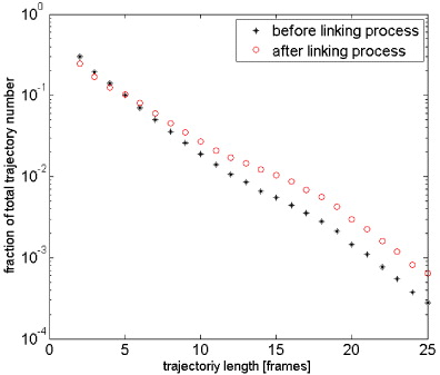
Figure 8. Refer to the following caption and surrounding text. — **Figure 8.** Typical histogram of trajectory lengths found in the PTV measurements before (black) and after (red) the trajectory reconnection procedure.
Download figure:
Standard image

In order to check the characteristics of short trajectories, table 1 contains the reasons why a two-frame trajectory (left) or a five-frame trajectory (right) is started (columns) or finished (rows), respectively. More than 65% of the two-frame trajectories are bounded by droplet images of very low intensity (category C in rows and columns), while this number is only 46% for the five frame trajectories. Of course, the probability of trajectories that are bounded by the real image borders increases with length: 78% of all five-frame tracks, while it is only 41% for two-frame tracks. The same applies to trajectories passing the out-of-focus limit (category B), which is more often observed for longer trajectories.

Table 1. Reasons (in %) for beginning (columns) and ending (rows) of droplet trajectories. Numbers indicate fractions of trajectories falling into each category. Left: two-frame trajectories; right: five-frame trajectories. A: out of image borders; B: out of focus; C: below intensity threshold; D: others.

4.4. Quantifying droplet collisions from tracking

The aim of the droplet tracking procedure is now to automatically identify situations that may involve a collision event, referred to in the following as a collision candidate. The process is designed to be semi-automatic due to the two-dimensional projection of the three-dimensional flow onto the image sensor. Even if a quantitative estimation of the depth position could be in principle derived from the intensity gradient of the droplet image, it does not allow a secure and fully automatic reconstruction of trajectories with the present setup. Thus, similar to the collision detection via the eccentricity measure using shadowgraphy [2], the PTV user is finally offered several collision candidates. It is left to the user to decide manually if a collision candidate is a valid collision or not. The detection of collision candidates uses a two-frame approach, in analogy with the tracking scheme itself. Specifically, the assumption of MA considering three successive frames is again considered. Two valid trajectories i,j in frames t − 1 and t have to fulfil the following conditions in order to count as a collision candidate:

their estimated future positions in t + 1, i.e. x^t+1_i = 2x^t_i − x^t−1_i and x^t+1_j = 2x^t_j − x^t−1_j have to be situated within the image borders,
the separation distance of their estimated future positions in t + 1 has to fall below a certain threshold, deduced from the radii of the droplet images, i.e. ∥x^t+1_i − x^t+1_j∥ < f_d(r_i + r_j), where f_d = 1.1 is an empirical factor measuring the required positioning proximity and
the separation distance of the positions in t and the estimated positions in t + 1 has to decrease, i.e. ∥x^t_i − x^t_j∥ > ∥x^t+1_i − x^t+1_j∥.

Typically, a complete set of 81 000 recordings delivered roughly 200 collision candidates, from which the end user had to identify real collision events.

Figure 9 shows an arbitrarily chosen, synthetic multiexposure image of ten PTV recordings (left) from which the droplet trajectories can be reconstructed (right). As can be seen, for instance in the lower part of the left image, droplets with too small intensity gradients and out-of-focus droplets are later excluded from processing. During this recording, one collision between droplets takes place within the measurement plane, i.e. the bold-plotted red and blue trajectories fulfil all conditions to be a collision candidate. Visual inspection confirms the detection, and a magnified image sequence of this specific event is presented in figure 10.

Figure 9. Refer to the following caption and surrounding text. — **Figure 9.** Left: synthetic multiexposure droplet image of ten PTV recordings; right: calculated trajectories of valid droplets for the same time period, including collision of two droplets (red and blue trajectories).
Download figure:
Standard image

Figure 10. Refer to the following caption and surrounding text. — **Figure 10.** Magnified time-history of the detected collision event from the time sequence of figure 9.
Download figure:
Standard image

5. Results

5.1. Characterization of the turbulent two-phase flow

In order to define the locations of the measurement points for LDV and PDA in the plane x = 0, a measurement grid was generated with 874 (19 in z-direction × 46 in y-direction) measurement points, with 10 mm distance in each direction between them. Since both LDV and PDA measurements provide high temporal resolution, the velocity components measured in the streamwise flow direction included the temporal fluctuations as well. All the measurement results are freely accessible through an Internet-based database (see www.ovgu.de/isut/lss/metstroem).

5.1.1. Laser-Doppler velocimetry measurements

LDV measurements with high temporal resolution are exemplified in figure 11 (left). From the autocorrelation function shown in figure 11 (right), the integral time scale can be estimated by $\int \rho (\tau )\,\textrm{d}\tau$ with τ∈[0,35] ms, resulting in a characteristic time for the integral scale of turbulence equal to τ_l = 7.45 ms for these conditions.

Figure 11. Refer to the following caption and surrounding text. — **Figure 11.** Exemplary time series of the axial velocity measured by means of LDV at point (x = 0, y = 150, z = 20) of configuration M4 (left). The mean flow velocity was 〈U〉 = 3.28 m s⁻¹ in this case. The associated autocorrelation function ρ(τ) is presented in the right picture, showing that ρ becomes negative after τ = 35 ms.
Download figure:
Standard image

Using Taylor's frozen turbulence approximation (∂/∂t = −u∂/∂x), LDV measurement data can be converted into a function of the spatial coordinate (r), since the fluctuation velocity is noticeably smaller than the mean flow velocity. It is then possible to calculate the second-order structure function of u(r) [67]:

$\begin{equation} S^{(2)}_u=\langle (u(x)-u(x+r))^2\rangle . \end{equation} \tag{ 16 }$

An exemplary result is shown in figure 12 for position (x = 0, y = 150, z = 120) of configuration M4. Although the inertial subrange is very narrow due to the low Reynolds numbers in the present flow, it is usually possible to apply a suitable linear fitting of the structure function. In this manner, it becomes possible to estimate the energy dissipation rate

$\begin{equation} \varepsilon= \left(\frac{S^{(2)}_u(r)}{2}\right)^{3/2}\frac{1}{r}. \end{equation} \tag{ 17 }$

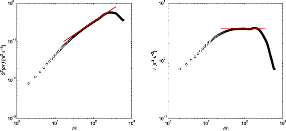
Figure 12. Refer to the following caption and surrounding text. — **Figure 12.** Second-order structure function as a function of the spatial lag calculated by means of Taylor's hypothesis (left). Using equation (17), the energy dissipation rate can then be determined by using a linear fit (right).
Download figure:
Standard image

Another alternative for the determination of the energy dissipation rate is spectral fitting. The LDV data have been reprojected onto an equidistant time series in order to derive a fast Fourier transform-based power spectral density (PSD) estimate [68]. Since the inertial subrange is narrow, a direct fitting by means of Kolmogorov's (−5/3) law would not be accurate. Therefore, two models [69–71] were used for a spectral correction. After an iterative fitting loop, the optimal fit was selected at each and every measurement point (see figure 13). Since the spectral estimation showed much less uncertainty compared to the structure function in most cases, the energy dissipation rate has been finally estimated systematically using the PSD of the LDV signals.

Figure 13. Refer to the following caption and surrounding text. — **Figure 13.** One-dimensional longitudinal velocity spectra as function of the dimensionless wavenumber × Kolmogorov length scale. The reconstructed inertial subrange is marked by the red line.
Download figure:
Standard image

Finally, the turbulent kinetic energy, the turbulent scales and the Reynolds number could be estimated for all cases. The corresponding results are summarized in table 2 for those measurement positions where the droplet collision rates were determined.

Table 2. Energy dissipation rate and derived turbulence parameters for all relevant measurement positions.

z-coordinates (mm)	ε (m² s⁻³)	u_rms (m s⁻¹)	k (m² s⁻²)	η_k (mm)	τ_k (ms)	Re_λ
M3
0	1.96	0.34	0.13	0.21	2.81	70
40	2.18	0.35	0.15	0.21	2.68	80
90	4.94	0.47	0.25	0.17	1.82	65
120	2.99	0.42	0.23	0.19	2.29	50
M4
0	1.73	0.21	0.09	0.22	3.01	30
20	2.82	0.21	0.08	0.19	2.36	30
40	2.35	0.24	0.11	0.20	2.58	40
60	2.82	0.41	0.21	0.19	2.36	100
90	7.11	0.62	0.46	0.15	1.48	140
120	4.54	0.50	0.30	0.17	1.86	110
140	4.26	0.26	0.10	0.17	1.92	30

5.1.2. Phase-Doppler anemometry measurements

PDA measurements have been conducted with the objective of characterizing the dispersed phase. The droplets have been measured independently from the continuous phase, at the same locations and for both configurations. Velocities measured by PDA are based on the same principles as LDV. However, using PDA the simultaneous measurement of droplet diameter and velocity is possible. Further properties such as the number of droplets per unit volume, the number of droplets of certain radii per unit volume, or the collision rate per unit volume, can be deduced by post-processing of the measurement data.

Measurements of droplet concentration have already been discussed by other groups [40, 41, 43, 72]. In the present work and based on PDA measurements, the droplet number density calculations by Roisman and Tropea [43] were applied in a slightly modified manner, as already described in section 3.2.2, allowing the calculation of the standard deviation and of the probability density function.

5.1.3. Collision probabilities

Collision probabilities have been determined from shadowgraphy as described in [33]. The algorithm is based on droplet shape analysis and discriminates collision events from aerodynamic droplet deformation, which would be an essential issue when considering large droplet diameters with Weber numbers larger than 1. This is not an issue in the present conditions. Different profiles were selected for the shadowgraphy measurements in the configurations M3 and M4, each in the x = 0 plane at y = 0 and y = 150 mm, respectively. The z-coordinates were in the range of z = 0 down to 140 mm.

After post-processing the experimental shadowgraphy results, a local collision probability p_coll was determined. This should now be converted into a collision rate, with the usual units of m⁻³ s⁻¹, by either using the data rate D or the droplet number density n. In [2], experimental collision rates have been documented using both approaches with nearly identical results, confirming the robustness of the procedure. It should be noted that the conversion by means of the droplet number density n showed a larger variability. Since an accurate determination of n is complex, as discussed before, the collision rate deduced from the direct quantity D is a logical choice. In what follows, the collision rate ( $\dot {N}_D$ ) is therefore systematically preferred. The standard deviation of the collision rates can be estimated using the same procedure.

5.2. Comparison between shadowgraphy and tracking

Now, a direct comparison is presented between collision probabilities obtained by shadowgraphy and PTV, two completely different approaches. In table 3, the collision probabilities are presented instead of collision rates or collision kernels, since this is the output directly obtained after post-processing combined with PDA measurement data, as already discussed before. The collision probability is defined as the ratio of the number of collisions to the total number of recorded droplets in the measurement section. The total number of droplets is easily obtained by shadowgraphy. For the high-speed PTV the total number of droplets is derived from the number of trajectories, as explained before. The total number of droplets for the determination of the collision probability is defined to be equal to the number of trajectories consisting of at least three steps. The shortest, two-frame trajectories have been neglected because the employed algorithm can never detect a collision from only two frames. Therefore, two-frame trajectories should be completely removed from the collision statistics.

Table 3. Measured collision probabilities p_coll of configuration M4 obtained by PTV (marked with ^P) or shadowgraphy (marked with ^S). The number of identified collision events N_coll and the total number of acquired droplets (or trajectories for PTV) N_tot are also included.

z-coordinate	N^P_coll	N^P_tot	p^P_coll	N^S_coll	N^S_tot	p^S_coll
0	N/A	N/A	N/A	3	28 542	1.05×10⁻⁴
20	N/A	N/A	N/A	5	43 647	1.15×10⁻⁴
40	1	146 440	6.83×10⁻⁶	3	30 046	1.00×10⁻⁴
60	5	145 447	3.44×10⁻⁵	4	30 941	1.29×10⁻⁴
90	8	177 057	4.52×10⁻⁵	8	27 284	2.93×10⁻⁴
120	2	99 787	2.00×10⁻⁵	6	28 711	2.09×10⁻⁴
140	3	122 659	2.45×10⁻⁵	2	18 986	1.05×10⁻⁴

It should be noted that the comparison is not based exactly on the same measurement recordings, since the magnification and therefore the field of view is different for both systems. Shadowgraphy can only be applied with good accuracy at high magnification, while PTV requires a minimum size of the measurement section in order to record enough positions for trajectory building. However, the measurements correspond to exactly the same conditions for the two-phase flow and are centered around the same position.

It can be seen in table 3 that the number of collision events is of the same order of magnitude for both PTV and shadowgraphy. However, the total number of acquired droplets deviates by a factor of about 5. This is partly due to the larger field of view associated with particle tracking. In addition, and considering the employed estimation for the total number of droplets, PTV might tend to overestimate it, in particular when many trajectories are split into fragments. The implemented reconnection tries to solve this issue, but works at most for two missing particle images between valid trajectories. Therefore, it is expected that PTV overestimates the number of droplets, for instance when a real trajectory meanders around the plane of focus. In contrast, shadowgraphy may well underestimate the total number of droplets since the background compensation procedure obviously eliminates very small droplets from the images. Therefore, it is expected that the real values would lie in between that obtained by shadowgraphy (lower bound) and that of PTV (upper bound).

Considering now statistics, PTV measurements build on 15 × 5400 image sets (with 5400 recordings taking 1 s), with at least 13 min break between two image series, as mentioned before. If the particles pass the measurement section in clusters, during which the collision probability increases, and if such a cluster is not detected because it has a characteristic period between 1 s and 13 min, the resulting statistics would be strongly influenced. However, there is in principle no reason to expect such clusters, all the control procedures working continuously and at short time scales.

Shadowgraphy acquires images at a constant pace, but with a recording frequency of merely 10 Hz. Assuming statistical stationarity this low frequency should not be a problem because the signal is averaged over many integral time scales. As a consequence, meaningful statistics are expected for both measurement techniques in the present conditions.

An obvious advantage of the high-speed PTV approach is the dynamic discrimination of collision events by considering sequences of consecutive recordings. This might be more reliable than the instantaneous approach used for shadowgraphy, where a collision can only be evaluated from one frozen recording. It cannot be excluded that sometimes, in particular due to the integrating character of the backlight illumination, a collision event will be mistaken for a droplet passing close to another one but at a slightly different depth. Figure 14 shows an example where the eccentricity value measured by shadowgraphy would have predicted a collision from any intermediate image in this sequence. Indeed, considering only for instance the third image in this sequence, a collision seems to be a realistic estimate. However, PTV reveals that both droplets indeed pass each other closely but without coalescence.

Figure 14. Refer to the following caption and surrounding text. — **Figure 14.** Image sequence of droplets passing close to each other as acquired by PTV.
Download figure:
Standard image

To summarize, it is expected that:

shadowgraphy delivers a lower bound for droplet numbers, while PTV delivers an upper bound;
shadowgraphy delivers an upper bound for the collision events, while PTV delivers a lower bound;
finally, the real collision probability found in the experiments should lie between that measured by PTV (lower bound) and shadowgraphy (upper bound).

5.3. Comparison with theoretical predictions

The resulting collision rates $\dot {N}_D$ estimated experimentally from shadowgraphy are now shown as blue triangles in figures 15 and 16. The independently estimated $\dot {N}_D$ from PTV measurements are shown for configuration M4 as pink triangles in figure 16. The error bars show the measurement uncertainty, which has been calculated using the standard propagation of uncertainty $\sigma _f^2 = \sum _i (\sigma _{x_i} \partial f / \partial x_i)^2$ . The calculation of the total collision rate is carried out by the formula

$\begin{equation} \dot{N}=\frac{N_{\rm{coll}}}{N_{\rm{tot}}}\frac{D}{V_{\rm{det}}}, \end{equation} \tag{ 18 }$

with N_coll the number of collisions, N_tot the total number of droplets, V_det the PDA detection volume and D the data rate. Since the standard deviation of the term $n_D=\frac {D}{V_{\rm {det}}}$ has been directly determined from the PDA measurements, the variance σ_{n_D} is directly involved in the propagation of uncertainty. The uncertainty of the total number of droplets and of the collision events is estimated by the Poisson counting uncertainty ( $\sigma _N=\sqrt {N}$ ). Thus, the uncertainty of the measurements can be calculated by

$\begin{equation} \sigma_{\dot{N}}=\sqrt{\left(\frac{n_D}{N_{\rm{tot}}}\sqrt{N_{\rm{coll}}}\right)^2 +\left(\frac{N_{\rm{coll}}}{N_{\rm{tot}}^2}n_D\sqrt{N_{\rm{tot}}}\right)^2 +\left(\frac{N_{\rm{coll}}}{N_{\rm{tot}}}\sigma_{n_D}\right)^2}. \end{equation} \tag{ 19 }$

It is important to note here that most of the measurement uncertainty is due to the fluctuation of the data rate D, i.e. the droplet number. The figures are plotted so as to mimic the geometric configuration of the wind tunnel measurements, with the (vertical) z-coordinate as ordinate, and the collision rate as abscissa (on a logarithmic scale). As discussed before, the collision rates from shadowgraphy are considerably larger than from PTV.

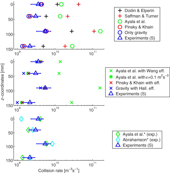
Figure 15. Refer to the following caption and surrounding text. — **Figure 15.** Theoretically predicted and experimentally determined total collision rates as a function of the vertical coordinate for measurement configuration M3. Experimental results from shadowgraphy are marked with triangles. In the upper panel theoretical approaches without efficiencies are marked by crosses (transport only) and circles (transport and accumulation). In the middle panel collision rates that include the corresponding collision efficiencies are denoted by ×. In the bottom panel results calculated with experimentally determined rms velocity fluctuations (*) are shown with diamonds.
Download figure:
Standard image

Figure 16. Refer to the following caption and surrounding text. — **Figure 16.** Theoretically predicted and experimentally determined total collision rates as a function of the vertical coordinate for measurement configuration M4. Experimental results are marked with triangles (blue for shadowgraphy, pink for PTV). In the upper panel theoretical approaches without efficiencies are marked by crosses (transport only) and circles (transport and accumulation). In the middle panel collision rates that include the corresponding collision efficiencies are denoted by ×. In the bottom panel results calculated with experimentally determined rms velocity fluctuations (*) are shown with diamonds.
Download figure:
Standard image

Also plotted in figures 15 and 16 are collision rates calculated for all theoretical expressions given in section 2. The comparison requires calculation of the theoretical collision rate from the measured size distribution and the collision kernel. Therefore, the corresponding collision rate equation is solved for each size pair obtained by discretizing the size distribution

$\begin{equation} \dot{N}= \sum_{i,j} \dot{N}_{i,j}=\sum_{i,j} n_i n_j \Gamma_{1,2}. \end{equation} \tag{ 20 }$

The resulting matrix is graphically presented in figure 17. Due to symmetry ( $\dot {N}_{i,j}=\dot {N}_{j,i}$ ), only one triangular half of the matrix has to be considered. Finally, the elements of one triangular part of the resulting matrix are summed up, including the matrix diagonal [73]. It is important to note that a threshold of 15 μm had to be applied for the minimum diameter, due to the spatial resolution of the experimental measurements. For this reason, the DSD was bounded by this lower value during the calculation of both the experimental and theoretical collision rates and collision kernels.

Figure 17. Refer to the following caption and surrounding text. — **Figure 17.** Collision rate matrix of the discretized DSD for the position (x = 0, y = 150, z = 90) of configuration M4.
Download figure:
Standard image

Binning in the tail of the PDF (equation (20)) is a subtlety that may have a noticeable influence on the calculated total collision rate. Despite the high number of droplets (typically at least 20 000, see table 3) that has been acquired at every single measurement position, the measured data are affected by sampling noise in the tail of the distribution. If the number of bins is decreased, the width of the bins increases and with that the number of droplets in each bin also does. But, on the other hand, the integration error also increases with the width of the single diameter classes. Using a linear binning, a bin width of 3.5 μm still leads to insufficient noise depression (figure 18). At the same time, even wider diameter classes would lead to much too coarse resolution in the peak region of the PDF. Therefore, it is clear that (i) the tail and peak regions of the PDF should be separately classified, and (ii) the tail region should contain increasing bin width with larger diameters. Therefore, the peak region (below 50 μm) of the PDF was spaced using a linear bin width of 1 μm in the present project, while the tail was discretized with a logarithmic bin spacing. Using such a logarithmic binning, the number of bins no longer has a noticeable influence on the results and 100 size classes already lead to a reasonable resolution within the complete tail region (see figure 18).

Figure 18. Refer to the following caption and surrounding text. — **Figure 18.** Influence of the bin width on the tail of the PDF for linear (left) and logarithmic (right) bin width. With decreasing bin number (increasing bin width) the noise reduces and the difference between theory and experiment is reduced.
Download figure:
Standard image

5.3.1. The theoretical collision rates

The theoretical collision rates calculated for the measurement conditions fall into several categories, and are therefore separated in several subfigures in figures 15 and 16 to avoid confusion. The top subfigures contain a comparison of just the transport and, where relevant, accumulation contributions to the collision rate, i.e. without collision efficiency. The pure gravitational kernel is shown as blue circles and, as expected, is less than all other theoretical expressions, which account for gravity plus turbulence. Collision rates calculated with the theories of Dodin and Elperin [4] (black +), Saffman and Turner [3] (red +), Ayala and co-workers (green circles), and Pinsky and co-workers (red circles), again all without collision efficiency, are shown for comparison.

The central subfigures in figures 15 and 16 contain a comparison of the collision rate expressions that take into account collision efficiency. Included are the theory of Ayala et al [6] together with the Wang and Grabowski [29] efficiencies (green ×), the theory of Pinsky et al [7] including their tabulated efficiencies (red ×), and the gravitational collision rate with the Hall [32] collision efficiencies (blue ×). For the Pinsky and coworkers calculation the energy dissipation rate of 1000 cm² s⁻³ is the value closest to the current experiments (but still too low), and has therefore been used for this comparison. Thus, in order to have a comparison of the collision rates with those of Pinsky and Khain, the Ayala kernels were calculated using a constant dissipation rate of 0.1 m² s⁻³ (green *). We also note that the Wang and Grabowski efficiencies are calculated only for radii up to 100 μm. For larger sizes, a value of 1 has been prescribed.

Finally, the lowest subfigures show the Abrahamson [23] expression with velocity variances calculated directly from the PDA measurements (light blue diamonds), as well as the theory of Ayala and co-workers with experimental results substituted in equation (9) (green diamonds). These latter cases do not include collision efficiencies.

6. Discussion and conclusions

Figures 15 and 16 are consistent in their comparison of measured and calculated collision rates. First, the theoretical collision rates are within a factor of 10 of the measured results, which is encouraging. Many of the theoretical values lie outside the uncertainty bars for individual measurements, but this must be interpreted with care. Remember that the collision rates derived from particle tracking shown in figure 16 are consistently lower than those from shadowgraphy by approximately a factor of 5–10. This trend, already explained previously, together with the calculated measurement uncertainties shown as horizontal error bars, suggest an overall measurement uncertainty of roughly a factor of 10, so that comparisons between theory and measurement should be interpreted in that context.

More generally, it can be stated at least qualitatively that the theoretical collision rates accounting for collision efficiency (middle subfigures) are noticeably closer to the measured values than those accounting only for transport and accumulation effects (top subfigures). A second general feature of figures 15 and 16 is that the gravity-only calculations are surprisingly close to the measurements, generally just below the shadowgraphy results, somewhat lower when the efficiency is taken into account. Further, the Pinsky and Khain and Ayala et al results that are calculated with ε = 0.1 m² s⁻³ are very close to the pure gravity results, suggesting a rather dominant role of gravity under those conditions, which is consistent with the observed presence of a large-droplet tail in the size distribution, with measurable concentrations of droplets greater than 100 μm (see figure 18). At the high dissipation rates measured, however, the contribution of turbulence to the collision rates can be seen to be significant. Of the theories calculated with the correct ε the Saffman and Turner result usually gives the highest collision rates. Indeed, Ayala et al stated that their transport term lies below that predicted by Saffman and Turner and by Dodin and Elperin. The fact that the Ayala collision rates are sometimes greater than those predicted by the Dodin and Elperin expression is a result of the additional inclusion of the accumulation effect. The possible overprediction of Ayala et al even when including the collision efficiencies (at the correct ε) is especially apparent in configuration M3 (figure 15). It is not completely clear yet which part of the theoretical formulation is responsible for this effect, i.e. either the relative velocity, through equations (8) and (9), or the accumulation effect through equation (10). It is possible that this discrepancy is associated with the largest droplets. Dodin and Elperin, Saffman and Turner, and Pinsky and Khain avoided this issue by essentially relaxing to a completely gravity-dominated collision kernel as drop size increases (explicitly for radii greater than 21 μm in the implementation of Pinsky and Khain). Finally, we compare the measured collision rates to more empirically calculated expressions, using the directly measured drop velocity variances. The results are shown in the bottom panels of figures 15 and 16, where the velocity variance is used in the Abrahamson expression as well as replacing the transport term in the Ayala et al expression. The agreement between measurements and the Ayala et al data is quite good, although it should be noted that the Wang and Grabowski efficiencies are not included here. Nevertheless, it provides an indirect suggestion that the transport term of Ayala et al may be overestimating the droplet relative velocities.

Several questions arise in interpreting the results. The theoretical calculations assume that drops are fully relaxed to the flow conditions and to their terminal fall speeds, whereas in the experiments the drops are injected in counter-flow with some initial velocity and require sufficient time for relaxation. The relaxation time, however, depends strongly on drop size [74]. The distance from the spray injection to the measurement plane is 540 mm, which through the mean wind speed translates to an advection time of 0.16 s. In fact much more time is available for relaxation because the injector is pointed upstream, i.e. the drops must relax to the flow in order to reverse direction and eventually reach the measurement volume. It should be pointed out that measurements of collision rates by observing changes in the shape of the size distribution are much more susceptible to such biases because they depend on integrated collision rates that may change due to variable turbulence conditions, etc. In this work, in contrast, the collision rate is observed directly in a small volume well downstream of the turbulence generation and spray injection. Another experimental challenge, as already mentioned, is the sensitivity of the results to sampling of the large-drop tail. All of these factors point to the importance of measuring with a narrower size distribution, both to reduce the relative importance of gravitational settling and to get more information on the size-dependence of the collision kernel. It is a nontrivial experimental task to produce very narrow drop size distributions in large number concentrations, so this remains as work for the future.

Acknowledgments

This project is part of the SPP1276 MetStröm and was financially supported by the German Research Foundation (DFG). RS acknowledges support from US National Science Foundation grant number AGS-1026123. Helpful discussions with H Xu and H Siebert concerning collision and turbulence processes are gratefully acknowledged. Furthermore, valuable guidance from L-P Wang, M Pinsky and A Khain regarding the implementation of their collision expressions is greatly appreciated.