


Abstract
We numerically calculate the optical conductivity of twisted graphene bilayers within the continuum model. To obtain the imaginary part, we employ the regularized Kramers–Kronig relation, allowing us to discuss arbitrary twist angles, chemical potential and temperature. We find that the Drude weight D as a function of the chemical potential μ closely follows the shell structure of a twisted bilayer displayed by the density of states. For certain angles, this results in a transport gap D = 0 at finite μ. We also discuss the loss function which, for low doping, is characterized by acoustic interband 'plasmons' and transitions close to the van Hove singularities. For larger doping, the plasmon mode of a decoupled graphene bilayer is recovered that is damped especially for small wave numbers.
Export citation and abstract BibTeX RIS

Content from this work may be used under the terms of the Creative Commons Attribution 3.0 licence. Any further distribution of this work must maintain attribution to the author(s) and the title of the work, journal citation and DOI.
1. Introduction
Since the realization that neutral graphene monolayers display a universal optical absorption of πα ≈ 2.3% in the infrared and visible spectrum (with α ≈ 1/137 the fine structure constant) [1–4], interest in the interactions between light and graphene has grown rapidly [5–7]. A remarkable aspect of this absorption, other than its suggestive relation to the universal constant α, is its high value, given the ultimate thinness of a graphene monolayer. In fact, it can be even enhanced up to 10% for photon energies around 4.5 eV due to transitions close to the van Hove singularity [8, 9].
The unique feature of neutral graphene responsible for its strong optical response is the existence of low energy particle–hole interband excitations with zero momentum, by virtue of the gapless Dirac spectrum, that act as an effective sink for photons of arbitrarily low energy. By the same token, all thermally excited plasmons in undoped graphene are damped by this excitation density, but nevertheless remain well-defined [10]. The unique bipolar tunability of graphene further allows one to adjust these optical properties quite simply, by shifting the Fermi energy μ away from the Dirac point, be it electrostatically or through chemical doping. This opens a gap of energy 2μ in the particle–hole excitations, making graphene transparent below this energy, useful, e.g. for broadband optical modulation [11]. It also allows for the emergence of undamped plasmons [12–16].
The spectral features involved in the unusual optical properties outlined above are also present in graphene bilayers [17]. These are often classified according to their stacking, which in the absence of strain have three possible (meta) stable configurations: AB'-type (or BA', also known as Bernal stacking), AA'-type and twisted. The former two are minimal stackings (unit cell with only four carbon atoms) in which half or all sites in opposite layers are vertically aligned, respectively. The twisted bilayer is the most generic type, and is defined by a relative rotation of angle θ between the two layers. Each of the three stacking types exhibits a different low energy electronic structure, although all three react strongly to light like the monolayer. The twisted bilayer, however, and in particular the case of low twist angles (around and below 1°), has the richest optical response, a consequence of its complex low energy spectral properties. The response, moreover, is highly tuneable through the angle θ, an additional control parameter not available in the other graphenes. As a striking example, the strong frequency-dependence of twisted bilayer conductivity and thus reflectivity leads to a visible coloration under white light, that varies with angle θ, of flakes on 100 nm thick SiO2, as recently observed experimentally [18].
In this work we study the optical response of twisted graphene bilayers at different twist angles and temperature responsible for this effect. We analyze its optical conductivity at and away from neutrality, the Drude weight and plasmon spectrum. Some of these aspects, specifically the real part of the conductivity, have been studied in recent works for large-angle twisted bilayers [19, 20]. We will make connection with these, and extend them into the low angle regime.
The paper is organized as follows. In section 2, we introduce the continuum model of twisted graphene bilayer and discuss the electronic structure. In section 3, we introduce the Kubo formalism and also comment on the regularization of the Kramers–Kronig relation for the conductivity, necessary in the case of unbounded Dirac fermions. In sections 4 and 5, we present our results for the optical conductivity and the related Drude weight for different angles, chemical potential and temperature. In section 6, we discuss the plasmonic spectrum based on the local conductivity by plotting the energy loss function and close with conclusions.
2. Continuum model of a twisted graphene bilayer
Twisted graphene bilayers are a peculiar structure from a crystallographic point of view, since for a generic (non-commensurate) angle the lattice is not exactly periodic, although crystalline order within each layer is extraordinarily robust. This is a consequence of the highly anisotropic binding forces in these systems, also characteristic of graphite. In principle only commensurate twist angles θ = θmn, where [21]

for integer m,n are amenable to band structure calculations by application of the Bloch theorem.
It turns out, however, that the bandstructure at low energies depends continuously on the value of the angle θn,m itself, not on the specific n and m (note that the set of possible commensurate angles θmn is dense). This is a consequence of the fact that the physical interlayer distance d > 0.3 nm is greater than the intralayer carbon–carbon distance acc = 0.14 nm. In this regime, all properties associated to precise commensurability are efficiently averaged out using microscopic tight-binding models. Consequently, a simple, low energy continuum theory can be formulated that may be applied to an arbitrary twist angle θ, and obviates all crystallographic complications to a very good approximation [21, 22].
The first ingredient in the continuum model is the momentum shift between Dirac cones in different layers due to the rotation, ΔK = 2|K|sin(θ/2), where |K| = 4π/3a0 and  is the monolayer Bravais period. The second non-trivial ingredient is the smooth spatial modulation in the interlayer coupling. The twist θ produces a triangular Moiré pattern in the local stacking, of period LM = a0/[2 sin(θ/2)], see figure 1(a). Hence, the coupling between layers becomes position dependent. The modulation is smooth on the scale a0, so the two valleys in each layer remain decoupled in the twisted bilayer. For each valley, the continuum model Hamiltonian reads [21, 23, 24]

This matrix is written in the local basis A,B,A',B' comprised of the two sites in the unit cell of each of the two layers. Here, the Fermi velocity is  and
and ![$\Pi _\pm =[k_x+\mathrm {i}(k_y\mp \Delta K/2)]{\mathrm { e}}^{{\mathrm { i}}\pm \theta /2}$](https://content.cld.iop.org/journals/1367-2630/15/11/113050/revision1/nj481264ieqn3.gif) . The function
. The function  describes the periodic spatial variation of the interlayer coupling, with γ⊥ ≈ 0.33 eV. The Moiré lattice vectors are denoted by a1,2 (so LM = |a1,2|) and conjugate momenta are g1,2, such that gi·aj = 2πδij (we also define g3 = 0). The AA' sublattice is centered at the origin, with the AB'/BA' sublattices offset given by
  . These offsets are used in equation (2) to write the sublattice-resolved interlayer coupling so that it alternates in space between AB', BA' and AA' types, following the Moiré pattern.

Figure 1. (a) Moiré pattern of a bilayer of index i = 15 (conf. equation (4)). Red hexagon denotes the Moiré unit cell. Panel (b) shows the corresponding low energy bandstructure, exhibiting a van Hove singularity at the M point around  = 0.02γ0. The eigenstates at these points are typically localized around the AA-stacked regions (inset in (a)). The transitions shown by arrows in (b) correspond to peaks in the optical conductivity marked in figure 3(b).
Download figure:
Standard image High-resolution imageWe first review the bandstructure phenomenology of the twisted bilayer. The continuum model has two distinct regimes, denoted as large and small angles, each with very different features. The large angle regime, relevant for θ greater than a few degrees, is characterized by two low energy Dirac cones per valley at the superstructure K and K', with a reduced Fermi velocity [25–27]

where α = γ⊥/6M is an expansion parameter that represents the dimensionless interlayer coupling and M(θ) = ℏvFΔK/2 = (2π/3)ℏvF/LM is the energy scale associated to the Moiré period LM. Also, a low-energy van Hove singularity at energy vH ≈ M − γ⊥/3, see figure 1(b), is created [23, 28–31].
At an angle θm1 ≈ 1.05°, known as the 'first magic angle', v*F becomes zero, the van Hove singularity degenerates into a narrow miniband around zero energy. This is the onset of the small angle regime. From this point on, the electronic structure becomes considerably complex. The Fermi velocity becomes finite again, as the miniband moves away from zero energy. Higher energy van Hove singularities appear and approach zero at subsequent magic angles θm2,3,4..., where the Fermi energy vanishes once more.
In figure 2, the density of states (DOS) is shown for various angles labeled by the index i

obtained from equation (1) with m = n + 1 = i. The curves are normalized by  such that the DOS of two uncoupled graphene layers is just a straight line with slope 1 (dashed line). Note that the DOS is almost but not exactly symmetric for positive and negative energies as a consequence of the underlying (not electron–hole symmetric) Hamiltonian.

Figure 2. DOS for different angles θi in units of  . Upper panel: θ = 3.15° (black) and θ = 2.13° (red). Lower panel: θ = 1.25° (black), θ = 1.05° (red) and θ = 0.91° (blue). The dashed and dotted-dashed lines resemble the DOS of decoupled bilayer and AA-stacked bilayer, respectively. The index i is related to the angle by equation (4).
Download figure:
Standard image High-resolution imageIn the upper panel, we show the DOS for 'large' angles θ with i = 10 (blue) and i = 15 (red). Around the neutrality point, the spectrum is characterized by a van Hove singularity followed by a step singularity, forming a closed shell. For small energies the system is thus approximately described by a hexagonal tight-binding model with renormalized band-width. This shell structure is somehow repeated for larger energies until it fades away and the DOS for decoupled bilayer graphene is recovered. Note that the weight of the van Hove singularity is slightly decreasing with increasing (intermediate) i.
For small angles around the first magic angle θm1 = 1.05° (i = 31, lower panel in figure 2), more distinct van Hove singularities appear and the height of the first van Hove singularity is strongly enhanced with increasing i. A close-up of this energy regime in shown on the left hand side of figure 8.
3. Linear response theory
The above phenomenology in the electronic bandstructure has an associated signature in the optical response of the system as the angle decreases. The basic quantity governing the linear optical response of any electronic system is the optical conductivity σαβ(ω) (where α,β = x,y), which gives the electric current arising in response to a weak and uniform, time-dependent electric field of frequency ω, E(t) = E(ω) eiωt,

The optical conductivity may be written, using linear response theory, in terms of the current response χjαjβ(q,ω) at zero-momentum,

where, as is conventional, δ denotes a positive infinitesimal. The current response function χjαjβ consists, in general, of two terms: the diamagnetic and the paramagnetic contribution [32]. The general formalism for obtaining the diamagnetic contribution in a tight-binding model is outlined in [33], however, in the continuum model for the twisted bilayer, as in the monolayer, the diamagnetic contribution vanishes due to the fact that ∂2H/∂k2α = 0. Hence, we have simply the paramagnetic contribution, given by the Kubo formula

Here, gs = gv = 2 are the spin and valley degeneracies. States |m,k〉 are eigenstates of H in subband m and of momentum k in the first Brillouin zone of the superstructure. Their eigenenergies are mk and nF is the Fermi function. The paramagnetic current operator is jα = −∂H/∂kα. In the continuum model with local interlayer coupling, this current does not mix layers and is thus independent of the coupling γ⊥. For a system with time-reversal symmetry, the conductivity tensor is diagonal and due to the threefold rotational symmetry of (twisted) bilayer graphene proportional to the unity tensor. We will, therefore, drop the tensor indices in what follows.
The real part of the conductivity σ(ω) represents the power dissipation of the system upon incidence of light at frequency ω, while its imaginary part represents inductive retardation of the current with respect to the driving field. From equation (6), it is obvious that the conductivity is ill-defined at ω = 0 and δ → 0 if χjj(q = 0,ω = 0) ≠ 0. It is thus customary to split up the conductivity into a regular part and a term containing the delta-singularity


with the Drude weight (or charge stiffness) D defined as

Above we used the fact that the imaginary part of the current response is an odd function. We thus have Im σ = Im σreg and will drop the subindex when confusion is unlikely.
3.1. Graphene monolayer
In the case of a graphene monolayer [34, 35], described within a continuum Dirac model, we have the famous zero temperature result (μ is the chemical potential with respect to the neutrality point)

This universal value σ0 for the Dirac gas includes valley and spin degeneracy factors, and is valid for energies ℏω ∼ 1 eV well below the γ0 ∼ 3 eV van Hove singularity of the monolayer. As ω approaches this scale, a discrete model must be employed to compute the monolayer σ0 (see [4] for general results).
The imaginary part of the conductivity, in the same limit of low frequencies, reduces to [3, 4]

where μ is the Fermi energy, measured from the Dirac point (charge neutrality). Using equation (10), we have a Drude weight

which vanishes at neutrality. Note that the above expression only scales with the chemical potential and no other material constant (Fermi velocity) is involved. The Drude weight for twisted bilayer as function of μ will thus be independent of the twist angle in the regime where the electronic spectrum can be described by a (renormalized) Dirac model. This breaks down close to the first magic twist angle with the emergence of a flat band.
3.2. Twisted bilayer
In the more general case of a twisted bilayer, the computation of σ(ω) becomes a numerical task and it is usually simpler to compute Re σreg than Im σ, since, by virtue of equation (7), the former reduces to an integral constrained to eigenstates within ℏω of the Fermi energy

The real part of the conductivity differs from that of two decoupled monolayers only at frequencies smaller than or comparable to the interlayer coupling ω < γ⊥. Hence we have Re σreg(ω ≫ γ⊥) ≈ 2σ0. This result will be useful in the following discussion to obtain a regularized expression for the imaginary part of the conductivity.
To compute the imaginary part, and from that, the Drude weight D through equation (10), one could in principle employ equation (7). This is problematic, since it involves a summation, even for small ω, over the whole band, which in the continuum model extends to infinity. We will, therefore, make use of the Kramers–Kronig (KK) relation, applicable to any response function. In terms of the conductivity, this yields

where  denotes the Cauchy principal value. There is apparently no advantage to using equation (15) as compared to equation (7), since the integral above extends to infinity, too. Moreover, the integral is ill defined, since at high frequencies the continuum model yields a constant Re σreg(ω ≫ γ⊥) ≈ 2σ0.
We will thus define the imaginary part relative to this divergent background following the usual procedure of ultraviolet field theories. In fact, this is one way of obtaining equation (17) and was discussed more generally in the context of the f -sum rule in [36]. The low energy properties are not modified by this regularization and we can simply subtract the ground-state expectation value of the two independent graphene layers at zero doping. Since the imaginary part for the neutral system is zero for the continuum model, the final regularized definition of Im σ simply reads

Numerically, equation (16) can be evaluated by introducing a finite cutoff Λ for which Re σreg(Λ) ≈ 2σ0. Integrating the second term involving the 'ground-state value' 2σ0 then yields the final formula

Note that this expression should be independent of Λ as it was obtained from equation (16). The extra terms compared to the original KK-relation (15) can be interpreted as the diamagnetic contribution that naturally arises in the Dirac model with finite band cutoff.
Using this expression, the Drude weight D in equation (10) may be written as

This expression, like equation (17), becomes Λ-independent for large cutoffs. In terms of D, equation (17) is then finally rewritten as

From equation (18), we can also deduce the f -sum rule

which is independent of the angle θ, chemical potential μ or temperature T.
4. Optical conductivity
The conductivity at neutrality μ = 0 is shown in figure 3 for two 'large' twist angles. Much like the monolayer, the real part (black) exhibits a universal asymptotic value Re σ(ω → 0) = 2σ0. It also exhibits signatures of the van Hove singularities, in form of a dip-peak structure as discussed in detail in [19]. The imaginary part (red) exhibits similar features, but vanishes at ω → 0, i.e. there is no Drude weight at μ = 0. This changes for finite temperature where the real part of σ is suppressed for  [37], as a consequence of the cancelation of the nF difference in equation (14). This results in a finite Drude weight, necessary to fulfill the f -sum rule equation (20). The Drude weight for finite temperature can be deduced from equation (13) with the substitution μ → 2 ln 2kBT [38]. Note that increasing temperature merely changes the Drude weight (figure 7), not the width of the Drude peak, i.e. Re σreg(ω → 0) = 0 at finite T. Temperature can further cause a shift of spectral weight close to the transitions associated to the van Hove singularity (see the circled region), creating new peaks that are absent at zero temperature.

Figure 3. Real (black) and imaginary (red) part of the optical conductivity of twisted bilayer graphene at neutrality μ = 0 for two different angles at T = 0 (i = 10, left and i = 15, right). Normalization constants are the universal monolayer conductivity σ0 = (π/2)e2/h, and γ0 = 2.78 eV. Index i is related to the angle by equation (4). The dashed lines refer to finite temperature with T = 300 K. Arrows on the right panel correspond to optical transitions in figure 1(b).
Download figure:
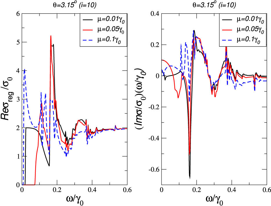
Standard image High-resolution imageIn the case of finite doping μ ≠ 0, see figure 4, the imaginary part of the conductivity develops a ∼ D(μ)/ω low frequency divergence, while the real part becomes suppressed below a threshold frequency 2μ for small enough μ (see black and red curves). Unlike for the monolayer, however, this is only true for μ below the van Hove singularity, since it relies on the linearity of the bandstructure (and DOS) around μ = 0. For chemical potentials close to the van Hove singularity, i.e. μ ≈ M, the optical gap is again filled by spectral weight and the Drude weight reduces consistent with the f -sum rule (blue dashed curves). At finite temperature, the optical gap may persist for small twist angle and the Drude weight can thus even increase, see figure 7.

Figure 4. Real (left) and imaginary (right) part of the optical conductivity at increasing value of the Fermi energy μ, as measured from neutrality for θ = 3.15° (i = 10). Rest of parameters like on the left hand side of figure 3. Note that Im σ(ω) has been multiplied by ω to reveal its ω → 0 asymptotics.
Download figure:
Standard image High-resolution imageFor large chemical potentials μ ≫ M, the electronic spectrum (DOS) of the continuum model is just that of two uncoupled graphene layers and one could thus expect to recover the conventional graphene conductivity. But the Moiré coupling between layers induces additional damping, since it opens up the possibility of more interband dissipation channels, i.e. any particle–hole excitation with momentum equal to a multiple of the momenta of the Moiré lattice. In order to understand the basic features of the conductivity on the basis of the uncoupled system, we can thus attribute a finite in-plane wavenumber q ∼ nΔK to the incoming photon (n > 0), see figure 5. The two-particle spectrum of interband and intraband excitations then predicts dissipation at low energies (black) and a broadened transition (blue) from the optical gap to the universal value 2σ0 of the conductivity.

Figure 5. Two particle spectrum of pristine graphene. Black shaded regions correspond to intraband transitions, whereas blue and violet shaded regions indicate interband transitions. The red vertical line denotes processes with finite momentum q.
Download figure:
Standard image High-resolution imageIn figure 6, the optical conductivity at the first magic angle i = 31 is shown for various chemical potentials (solid lines) and compared to Re σreg for i = 10 (dashed blue line). For low chemical potential, the optical response differs considerably for small and large angles, but for increasing μ the dependence on the twist angle becomes less and Re σ is characterized by a large Moiré-broadening of the optical gap around ℏω = 2μ. Still, there is the pronounced spectral weight at ℏω = vH almost independent of μ, which is especially striking for larger angles. This feature cannot be explained from figure 5 and is twist angle dependent.

Figure 6. Real (black) and imaginary (red) part of the optical conductivity for different chemical potential μ at the first magic angle θm1 = 1.05° (i = 31). Rest of parameters like in figure 3. For comparison, also Re σ for (i = 10) is shown (dashed blue line). Dotted lines resemble the limit for uncoupled layers. Note that Im σ(ω) has been multiplied by ω to reveal its ω → 0 asymptotics.
Download figure:
Standard image High-resolution image5. Drude weight
Considering only intraband transitions of one unbounded conduction band, the Drude weight or charge stiffness is proportional to the chemical potential, independent of its dispersion relation. For parabolic band electrons, D is thus simply related to the charge density, D = e2n/m, whereas for Dirac Fermions one gets  , see equation (13). In systems with a finite band-width, we expect a non-monotonous behavior expressing the fact that the Fermi energy is first related to electrons and later to holes when sweeping the chemical potential through the band. For the one-dimensional tight-binding model, one finds, e.g.
  with 2γ0 the band width. For the two-dimensional (2D) hexagonal tight-binding model, the system is characterized by a van Hove singularity at μ = γ0 around which the Drude weight shows a maximum [37].
For twisted bilayer graphene described by the continuum model, we expect a combination of both features, because of the unbounded linear dispersion of Dirac Fermions and the superlattice structure of the Moiré-pattern. From figure 2 we see that the DOS is characterized by a van Hove singularity followed by a 'real' step-like singularity which is repeated to higher doping levels. This pseudo-gap structure divides the spectrum in several bands and will be followed by the Drude weight. Nevertheless, these modulations are superposed onto a constant linear background as suggested by the unbounded continuum model.
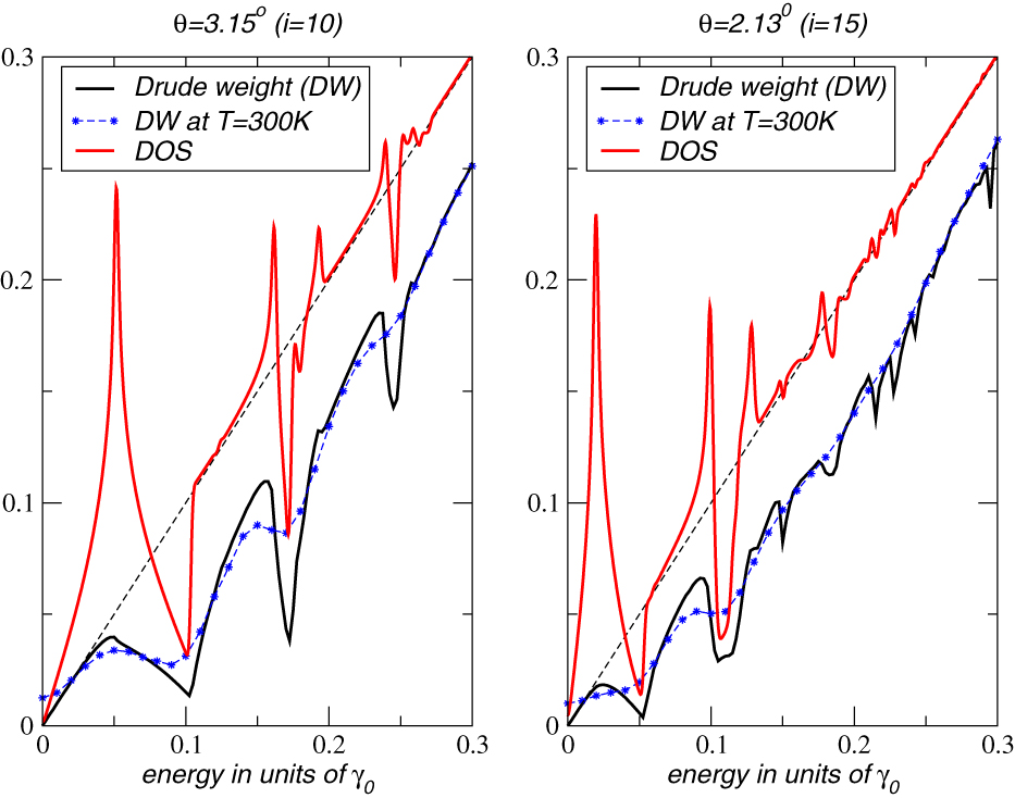
The μ dependence of the Drude weight D(μ) in units of 2D0 is presented in figure 7 for two large twist angles. As is apparent, for small chemical potential D(μ) follows twice the monolayer value 2D0 independent of the twist angle, as expected for Dirac systems. For larger μ, the Drude weight drops and remains less than 2D0 until it converges to the uncoupled bilayer system for μ ≫ γ0.

Figure 7. Drude weight D as a function of chemical potential μ for two different twist angles (black curve), together with the corresponding DOS (red curve). The thin dashed line corresponds to the Drude weight and DOS of two decoupled monolayers, in units of 2D0, equation (13), and  , respectively. Symbols (blue ⋆) resemble the Drude weight at T = 300 K.
Download figure:
Standard image High-resolution imageAs outlined above, D(μ) exhibits dips that accurately correlate with dips in the DOS, also shown in figure 7 (red). The resulting picture suggests the above mentioned approximate shell structure, albeit (in general) without gaps between shells, just as the suppressed DOS. The first shell can be fairly well approximated be the hexagonal tight-binding model.
At finite temperature T = 300 K (and also for disorder), the Drude weight is smeared out for large twist angle i = 10, thus reaffirming the interpretation of the repeated shell-structure. Nevertheless, the shell structure becomes less pronounced with smaller θ which is also reflected by its temperature response.
For small angles, the Drude weight provides a sensitive fingerprint for the breakdown of Dirac physics that occurs around the magical angles due to the emergence of flat bands. This can be seen on the right hand side of figure 8 for small angles above (i = 26) and below (i = 36) the critical angle. The Drude weight becomes larger than the Drude weight of two monolayers before it drops indicating the band width of the flat band. At the critical angle (i = 31), this band width becomes zero, and interestingly, the scaling of D0 is recovered. Note that for i = 26, we find a transport gap D = 0 at finite chemical potential μ = 0.06γ0.
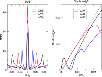
Figure 8. The DOS (left) and the Drude weight (right) around the first critical angle θ = 1.05° (i = 31) in units of figure 7. Dashed lines correspond to uncoupled bilayer.
Download figure:
Standard image High-resolution imageThe increase of the band width for twist angles larger than θm1 can be nicely appreciated from the Drude weight. This becomes considerably more difficult from the DOS, displayed on the left hand side of figure 8. The reason for this is that the Drude weight is obtained from integrating over the whole spectral region and not only from the low energy band structure. Nevertheless, the weight of the peak at zero energy is maximal at the magic angle (red curve), indicating its singularity.
6. Plasmons
A complementary aspect to the optical absorption is the plasmon excitation spectrum of the electron gas. Conceptually, a plasmon is an oscillating charge density mode (hence accompanied by an oscillating electric potential), which is sustained by the Coulomb interactions between electrons. The dispersion relation of these modes is given by the zeroes of the dielectric function (q,ω) = 0, that relates the screened electric potential Vsc(r,t) to an externally applied potential Vext(r,t),

A plasmon is, therefore, a finite solution Vsc(q,ω) that requires no external driving, i.e. it is self-sustained. A Landau-damped plasmon corresponds to a peak in 1/(q,ω), and decays due to dissipation into particle–hole excitations.
The dielectric function (q,ω) may be computed within the random phase approximation (RPA). In the long-wavelength limit, we may thus relate RPA directly to σ(ω) using equation (6),

where αg = e2/(4π0ℏvF) ≈ 2.2 is graphene's fine structure constant. In equation (21) we have neglected corrections due to the finite interlayer distance, and consider that interlayer and intralayer electron–electron interaction are of the same form ∼ 1/q. In this approximation all the collective modes correspond to charge excitations in which the charge oscillates in phase in the two layers [39, 40].
To compute ωp for small frequencies, we may expand Im σ in equation (19) by the Drude term,  . This results in the dispersion of a classical 2D plasmon

For two decoupled monolayers, one just replaces D = 8μ/πℏσ0 above, which is shown as dotted curved line in figures 9 and 10.

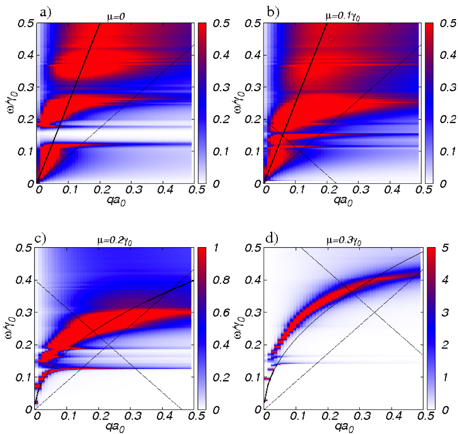
Figure 9. Loss function S(q,ω) = −Im −1(q,ω) in the long-wavelength RPA approximation for θ = 3.15° (i = 10) and = 2.4. The dashed curved line corresponds to the undamped plasmon of the decoupled bilayer. The region of undamped plasmons of the decoupled bilayer is defined by straight lines.
Download figure:
Standard image High-resolution image
Figure 10. Loss function S(q,ω) like in figure 9, for the first magic angle θ = θm1 = 1.05° (i = 31) and = 1.
Download figure:
Standard image High-resolution image
6.1. Plasmons in twisted bilayer
In twisted graphene bilayer there may exist four types of plasmonic modes or resonances: (i) undamped (conventional) graphene plasmons for chemical potentials with μ ≪ M; (ii) interband 'plasmons' present also for μ = 0; (iii) damped plasmons for large chemical potential μ ≫ M; and (iv) transverse plasmons. Below, we will briefly outline the main properties of these different types.
6.1.1. Undamped plasmons
At low doping, there exists a low energy window with Re σ = 0 that gives rise to undamped plasmons governed by the Drude weight D. In this regime, the twisted bilayer can be described by linear Dirac Fermions and D(μ) follows the Drude weight of the uncoupled system 2D0, as shown in figure 7. This energy window becomes smaller for decreasing twist angle since the van Hove singularity moves closer to the neutrality point and is only relevant for large angles.
6.1.2. Interband plasmons
In monolayer graphene, a peak in the loss function associated to π → π* transitions around the van Hove singularity and with linear dispersion was first predicted by DFT-studies [41], and later experimentally observed in suspended graphene by electron energy-loss spectroscopy [42]. Within the hexagonal tight-binding model and RPA, i.e. without including correlation or renormalization effects, no zero of the dielectric function is obtained [43]. The absorption peak would thus be merely due to interband transitions enhanced by a band-structure effect; nevertheless, in bi- or multilayer, RPA(q,ω) becomes zero around the M point [44]. In the twisted graphene bilayer, there exist several van Hove singularities such that interband plasmons (or absorption enhancement) are to be expected. These are especially dominate for large twist angle and can lead to a broad optical gap in the interband excitations where Im σ < 0.
6.1.3. Damped plasmons
In the regime of large chemical potential, μ ≫ M, the conventional intraband plasmon is recovered, albeit Moiré-damped. This can be deduced from figure 6 which will be used to discuss the plasmon dispersion in terms of the loss function. The dispersion only depends slightly on the twist angle and becomes well-defined for large μ, extending into the Landau damped region just as for the monolayer.
6.1.4. Transverse plasmons
There is also the possibility for transverse or transverse electromagnetic (TE) plasmons modes given by the condition [45]

For TE modes, the plasmon dispersion is closely pinned to the light cone which justifies our local approximation (q → 0) and there are (damped) solutions to equation (23) if Im σ < 0. Since they can only exist in twisted bilayer surrounded by a homogeneous dielectric background [46], we will not discuss them any further.
6.2. Loss function
The loss function, defined as S(q,ω) = −Im −1(q,ω) is a measure of the spectral density of plasmon excitations. Thus, a sharp peak in S(q,ω) reveals a long-lived (transverse magnetic (TM)) plasmon of that frequency and momentum. A proper undamped plasmon, defined by (q,ω) = 0, corresponds to a delta peak in S(q,ω), since −1(q,ω) satisfies Kramers–Kronig relations.
In figure 9, we present S(q,ω) within the long-wavelength RPA approximation of equation (21) at intermediate angle θ = 3.15° (i = 10) for different chemical potential with = 2.4. In figure 10, the same quantity is shown at the first magic angle θ = θm1 = 1.05° (i = 31) with = 1. In all plots, the Dirac dispersion ω = vFq and the ℏω = 2EF − ℏvFq from figure 5 is shown as dashed lines, indicating the onset of intra- and interband transitions.
The qualitative features of the plasmon spectrum in both behavior can be deduced from figure 6. For zero or low chemical potential (figures 9(a) and 10(a)), the loss function reveals an acoustic interband 'plasmon' with sound velocity vs ≈ παgvF/ (solid line). It is not a plasmon in the conventional sense, since the dielectric function does not become zero. This linear (interband) mode crosses over to the conventional  (intraband) mode, figures 9, 10(b) and (c), and becomes well-defined for large chemical potential, figures 9, 10(d), although there are slight variations compared to equation (22) shown as solid curved line. Note that for twisted bilayer on a substrate (e.g. ≈ 2.4), the local approximation of the conductivity needs to be improved for large chemical potential and low twist angle since there is considerable weight of the plasmon mode in the intraband particle–hole continuum for large q. In single-layer graphene, this is forbidden due to the square-root singularity of σ(q,ω) at ω = vFq.
The loss function also exhibits a pronounced optical gap in the region where Im σ < 0. This feature is especially visible at larger angles (figure 9). The gap is a consequence of the van Hove singularity, and is perhaps the most visible effect on the plasmon response of the Moiré pattern at large θ. Secondary van Hoves give rise to additional gaps at higher frequencies. At smaller angles, the gap is smaller and less defined, although some hints of it persist down to the first magic angle, specially close to μ = 0 (figure 10(a)).
7. Conclusions
We have analyzed the DOS, optical conductivity, Drude weight and plasmon spectrum in a twisted bilayer for various angles, doping levels and temperature, and compared them to the uncoupled system. We have found a universal low-frequency conductivity and peaks at finite frequency that correlate to van Hove singularities in the DOS. These latter features, however, become scrambled at decreasing angles. We have also shown that the Drude weight in twisted bilayers is usually below that of two decoupled monolayers, 2D0, and exhibits a shell-like structure, following again van Hove singularities in the DOS. Only for small angles close to the neutrality point, the Drude weight becomes larger than 2D0, signaling the emergence of a flat band. The Drude weight resembles a sensitive quantity to numerically distinguish the different electronic structure at critical angles since it is obtained from integrating over the whole spectrum and is directly related to transport experiments. We have finally discussed how plasmons may become damped by the interlayer Moiré coupling which opens up new dissipation channels. Significant spectral structure survives, however, including undamped plasmons and multiple long-lifetime resonances (interband plasmons) within the extended interband particle–hole continuum.
Acknowledgments
We thank G Gómez-Santos and E Prada for discussions. This work has been supported by FCT under grants PTDC/FIS/101434/2008; PTDC/FIS/113199/2009, by MIC-Spain under grant FIS2010-21883-C02-02, FIS2011-23713 and FIS2012-33521, and by the European Research Council Advanced grant, contract 290846.