


Abstract
Few-femtosecond to attosecond electron pulses are required for advancing ultrafast diffraction and microscopy to the regime of electrons in motion. Here, we report the combination of a single-electron source with a microwave cavity for pulse compression. In such an arrangement, the electron pulses can become significantly shorter than the laser pulses used for electron generation. This comes at the expense of an increase in energy spread. We report the use of an energy analyzer for characterizing microwave-compressed single-electron pulses. Phase effects, linearity, focal distances, incoming pulse durations and laser–microwave jitter are measured for three different synchronization approaches. The results demonstrate the applicability of a microwave cavity in the single-electron regime and identify jitter as the current limitation on the way to few-femtosecond, eventually attosecond pulses of single electrons.
Export citation and abstract BibTeX RIS
1. Introduction
Probing ultrafast dynamics of matter with ultrashort electron pulses at 30–300 keV can provide a dynamical, four-dimensional (4D) picture of atoms in motion. This is made possible by picometer-scale de Broglie wavelengths of electrons, which are about ten times shorter than atomic distances and highly suitable for diffraction. Structural dynamics can either be imaged directly by ultrafast 4D electron microscopy [1] or studied by diffraction in reciprocal space [2–4]. Many recent results demonstrate the ability of these laser-pump/electron-probe techniques to provide a largely complete, dynamical picture of atomic motion [5–8] or processes on nanometer/picoseconds scales [9–12].
Ultrashort electron pulses for 4D imaging are usually generated at a thin metal layer by photoelectric emission with a femtosecond laser. An electrostatic field is used to accelerate the electrons to their final energy. One or more magnetic lenses, ideally of 'isochronic' type [13], are used to collimate or focus the beam to the sample and screen. In order to obtain dynamical images or diffraction patterns with satisfactory signal to noise, a large number of electrons (typically >107) must be collected for each point in time at which the transient structure shall be determined. This can either be achieved by individual exposures with dense packets, or by repetitive pump–probe measurements at the same time delay with electron pulses of low density or single electrons [1, 14]. An intermediate pump/probe rate (about 0.5–5 MHz) is convenient in the latter case [15]. The type of dynamics under investigation, irreversible or reversible, determine the applicable method.
In dense electron packets, which are required for measuring irreversible or partially reversible processes, Coulomb repulsion is a major source of temporal broadening during propagation [16–17]. With electrostatic acceleration schemes, femtosecond resolution then requires an extremely short distance between source and sample [4] or energy filtering [18]. An alternative concept is pulse compression with a microwave cavity; this was first considered for electron diffraction in [19–20]. Time-dependent longitudinal electric fields are used to decelerate leading electrons and to accelerate trailing ones; this compresses the pulses at some location behind the microwave cavity. Pulses with 106 electrons, dense enough for single exposures, could recently be compressed to ∼100 fs with this approach [21], offering sufficient resolution for a range of atomic motions.
Electronic motion on the atomic scale, however, can evolve on time scales of a few femtoseconds and below. Advancing 4D imaging into this novel regime [22–24] requires electron pulses of, ideally, attosecond duration. Single-electron packets offer this potential owing to the absence of space charge. In this limit, the 'effective' pulse duration can be defined in terms of and determined from the statistical distribution of the arrival times of individual electrons at the sample, with respect to the excitation triggered by the pump-laser pulse [14].
At keV energies and de Broglie wavelengths of picometers, Fourier limits (uncertainty principles) impose no significant limitation to achievable pulse durations even down to regimes of a few attoseconds and below [25]. Practically, however, even single-electron pulses are not as short as desirable. Mismatch of the photoemission laser's photon energy and the photocathode's work function, inhomogeneities of the surface, and the bandwidth of the optical femtosecond pulses contribute to a shot-to-shot variation of energy and therefore arrival time, producing extended pulse durations at the sample [14]. Most fundamentally, pulses generated from a photocathode cannot be shorter than the optical femtosecond pulses used for photoemission. Advancing electron pulse durations into the few-femtosecond and (eventually) attosecond regime therefore requires additional concepts, beyond single-electron sources.
In this paper, we present our concept and first experimental results with a microwave cavity intended for compressing single-electron pulses to durations approaching 10 fs and possibly below. Firstly, we describe the general layout of our experiment. Secondly, we explain why we expect compression in the single-electron regime. Thirdly, we discuss the design of the cavity and laser-microwave synchronization. Fourthly, we show how we use an energy filter for diagnostics and analysis of jitter between the microwave and laser fields. We conclude with an assessment of the pulse durations achieved so far, and present our approaches for further improvements.
2. Experimental arrangement
Our concept for pulse compression is based on combining a single-electron source with electrostatic acceleration [14] with a microwave cavity for pulse compression [20]. In the single-electron regime, compression applies to the effective pulse duration of the electrons, i.e. the statistical distribution of their arrival times [14], with respect to the phase of the microwave field (see figure 1(a) and section 3).
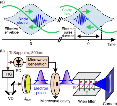
Figure 1. Concept and setup for single-electron compression. (a) Depicted are two single-electron pulses (light blue) and the microwave field (green). As a consequence of the photoemission process [14], the individual electrons (blue) can be located earlier or later within the effective pulse duration (dotted). The cavity field is used to compensate for this effect and to produce pulses significantly shorter than initially (see text). (b) Experimental arrangement. The output of a Ti:sapphire femtosecond laser is frequency-tripled (THG) and passes a variable delay (VD). Photoelectrons are generated from a 50 nm thick gold layer (yellow) and accelerated in a static potential Uacc. A photodiode (PD) and three different types of microwave synthesizers are used for synchronization. The electron pulses (violet) have a duration limited by the laser's pulse duration and the dispersive effects of the emission bandwidth. A microwave cavity is used to accelerate trailing parts and to decelerate leading parts, in order to compress the electron packet in time. An energy analyzer (Wien filter) with crossed electric and magnetic fields (E and B, respectively) is used for investigating phase effects, pulse durations, laser–microwave jitter, focal distances and linearity of the time–velocity relation (see text).
Download figure:
Standard imageThe experimental arrangement is depicted in figure 1(b). A Ti:sapphire oscillator provides 50 fs pulses at 800 nm with pulse energies of ∼500 nJ at a repetition rate of 5.128 MHz. This repetition rate is chosen to maximize the pump–probe rate, while providing enough time between the pulses for sample relaxation. The laser's operating principle is mode-locking via a saturable Bragg reflector in a long cavity [26]. This provides enough pulse energy for sample excitation and still sufficient stability of the repetition rate for microwave synchronization (see section 4).
For the following experiments, we use two weak fractions of the laser's output, while the main power is reserved for sample excitation. About 10 mW of the laser impinges on a very fast photodiode, in order to provide a signal for microwave synchronization (see section 5). Another ∼0.1 W are frequency-tripled (THG) with two thin β-barium-borate crystals and a delay plate. The resulting ultraviolet pulses at ∼266 nm are attenuated to the energy level of ∼20 pJ and focused on the photocathode (yellow), which is a 40 nm gold film on a thin quartz substrate. The gold layer is connected to an electrostatic potential of Uacc = −25 kV. Photoelectric emission generates single electrons (∼0.1 on average), which are accelerated in the static electric field toward the grounded casing of the microwave cavity. The microwave cavity is 'omega-shaped', i.e. toroidal with a radial cross-section resembling the letter 'Ω'. It supports the TM010 mode, having longitudinal electric fields that decelerate leading electrons and accelerate trailing ones, as depicted in figure 1(a). The cavity's resonance is driven by a microwave generator that is phase-locked to the laser's repetition rate (see section 5). After passing the microwave cavity, the electron pulses enter an energy analyzer, consisting of crossed electric and magnetic fields, also referred to as a Wien filter (see section 6). A camera (CMOS technology, 4096 × 4096 pixels, TVIPS GmbH) is used to record the electron beam or its energy spectrum. The ultraviolet part of the laser beam, which generates the electron pulses, can be delayed (VD), in order to adjust the relative timing between the electron pulses and the microwave's phase inside the cavity. All components involving electron beams are in high vacuum (∼10−6 hPa). For laser–microwave synchronization, we apply three different schemes, two based on phase-locked loops and one based on the direct amplification of the laser's frequency comb (see section 5).
The setup of our experimental apparatus reproduces quite closely the dimensions considered in the previous theoretical work [20]. The simulations there had predicted that final pulse durations of <1 fs could be achievable, provided a good-enough synchronization between the laser and microwave is realized.
3. Pulse compression of single-electron packets
Static approaches for electron pulse compression include reflectrons [27–28] and magnetic chicanes [29]. These arrangements can compensate for dispersion and re-compress the pulses down to their initial duration, but not further. A reduction of pulse duration below the initial value at the source, i.e. the duration of the femtosecond laser pulse, is generally not possible with static compression schemes. In contrast, a microwave cavity in combination with single-electron pulses promises reach into the few-femtosecond regime [19–20].
How can a microwave cavity possibly compress electron pulses to a duration much shorter than the optical pulses used initially for electron generation (∼50 fs)? Simulations predict sub-femtosecond durations [19–20, 25]. We invoke here an argument based on the conservation of volume in phase space. Figure 2 illustrates four essential stages of the electron packet in the time–velocity domain; lateral dimensions and relativistic effects are neglected. At the photocathode, electrons are generated during all of the laser pulse's duration (τinitial ≈ τlaser). In addition, the physics of the emission process [14] at our wavelength of 266 nm results in a bandwidth of ΔEinitial ≈ 0.2 eV. The initial phase space has therefore a width in time and a velocity spread; an approximation of such a packet is shown in figure 2 in grey. Note that this packet is depicted as if acceleration to the final energy (25 keV in our case) was instantaneous. Vacuum is highly dispersive for non-relativistic electrons; higher-energy electrons travel faster than lower-energy ones (red arrows). During propagation toward the cavity, the phase space therefore experiences a shear. Just before the cavity, faster electrons are in front of slower ones, and the pulse has a total duration τdisp (red phase space). In best cases, τdisp ≈ 80 fs [14]; with the lower acceleration fields used here we have τdisp ≈ 600 fs (see section 11). Note that in the single-electron regime no additional dispersive forces are induced by space charge; the bandwidth of ΔEinitial ≈ 0.2 eV is maintained (horizontal dotted lines). Next, the electron packet passes the cavity and its time-dependent fields: leading electrons are decelerated and trailing ones are accelerated (green arrows); the effect is linear in time if the microwave's period is much longer than the electron pulse's duration. More velocity change is applied than required to reverse the effect of dispersion. Accordingly, the pulses obtain an increased energy bandwidth, which significantly exceeds that of the initial packet. After the cavity, the dispersion of vacuum (blue arrows) acts to compress the pulses down to a duration τfinal at a temporal focus.
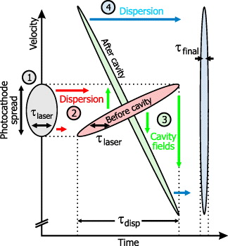
Figure 2. In the single-electron regime, the cavity can compress the electron pulses to durations much shorter than the laser pulses used for photoemission. This is possible by increasing the energy spread to values higher than the initial ones. The figure depicts the four essential steps of this process in phase space. For explanation, see text.
Download figure:
Standard imageApproximately, all four steps conserve the volume of phase space. Therefore, the initial and final pulse durations relate inversely proportional to the respective velocity spreads: τinitial Δvinitial ≈ τfinal Δvfinal, or approximately at large central energies, τfinal ≈ τlaser ΔEinitial/ΔEfinal. For example, at 30 keV, which is practical for ultrafast diffraction, we can allow for an energy spread of ΔEfinal ≈ 200 eV at the sample. The de Broglie wavelength has a spread of <1% in this case and the sharpness of Bragg spots is maintained. For our experimental settings with τlaser ≈ 50 fs and ΔEinitial ≈ 0.2 eV, final electron pulses could ultimately be as short as τfinal ≈ 50 as. Imperfections and nonlinearities in the transformations of phase space, for example spatio-temporal couplings in magnetic fields [13], the nonlinear effects of a limited acceleration strength or roughness of the cathode, can set higher limits. The general picture derived here, however, is instructive in order to understand the mechanism of temporal pulse compression in the single-electron regime.
4. Design of the microwave cavity
A central problem with microwave compression is that synchronization between laser and microwave is required [19–21]. On the one hand, in pump–probe experiments, the laser determines the instant of sample excitation. On the other hand, the electron pulses arrive at the temporal focus with a timing that is determined by the microwave's phase (see section 10). As a consequence, a jitter between the laser and the microwave's phase reduces the temporal resolution of a pump–probe experiment (by increasing the effective electron pulse's duration, defined above).
Synchronization can either be achieved by phase-locking the microwave to the laser or vice versa. We chose to let the microwave frequency follow the laser's repetition rate, which is stable over many hours within a few Hz at about 5.128 MHz (figure 3(a)). Figure 3(b) shows the laser's phase noise at higher frequencies, measured with a spectrum analyzer (PSA E4447A, Agilent) that has a clock stability of better than 5 × 10⁻⁷. Accumulated from the Nyquist frequency to 10 Hz, the jitter between clock and laser is less than a few ps. The phase noise shows strong components only at acoustic frequencies in the range below 500 kHz; above, the measurement is limited by the analyzer's dynamic range and the quality of its clock.
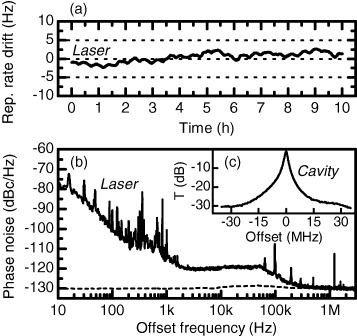
Figure 3. Drift and jitter of our long-cavity laser source at 5.128 MHz. (a) The repetition rate changes by only a few Hz over several hours. (b) The laser's phase noise shows strong contributions only at acoustic frequencies below ∼500 kHz. (c) The resonance of the microwave cavity at a central frequency of 6.2 GHz is designed with a width of ∼2 MHz, corresponding to a quality factor of ∼3100. Plotted is the transmission T measured at the cavity's output port (see text).
Download figure:
Standard imageThe cavity's resonance was designed according to these findings. A high quality factor (i.e. narrow bandwidth) is beneficial to generate the required electric fields for electron compression at lowest input power. However, a minimum of bandwidth is required to account for the laser's fluctuations and drifts. Moreover, too a high quality factor causes a steep phase change as a function of frequency around the cavity resonance. A small frequency drift can lead to a significant phase change of the microwave field inside the cavity, and therefore reduce the quality of synchronization. These considerations and the laser parameters lead to an optimum cavity bandwidth of a few MHz.
A second parameter is the cavity's central frequency. We chose a rather high value of 6.2 GHz. This is beneficial for two reasons. Firstly, synchronization is facilitated, because a lower accuracy of phase-lock is sufficient at higher frequencies for achieving the same timing jitter. Secondly, the power required to drive the cavity is reduced, because the temporal slope of the electric field determines the strength of electron pulse compression, i.e. the amount of induced velocity spread and the position of the temporal focus. The cavity's effect can be described by a time-dependent acceleration parameter gv = Δv/τdisp, or alternatively by a time-dependent energy gain gE = ΔE/τdisp, where  , Δv and ΔE are the incoming packet's duration, and the outgoing packet's velocity spread and energy spread, respectively. In the non-relativistic case, we obtain for the distance of the temporal focus, f:

where v0 and E0 are the incoming packet's central velocity and central energy, respectively, and me is the electron's mass. Because gv and gE are proportional to the change of the field with time, and the required power is proportional to the square of the field's amplitude, higher microwave frequencies require significantly less power for achieving the same focal distance and compression. A specific formula is reported in [20].
However, the upper resonance frequency is limited by the feasible physical dimensions of the cavity and the availability of low-noise/high-frequency equipment. In addition, the period of the microwave field must be considerably longer than the length of the incoming electron pulses (τdisp), in order to achieve a linear temporal slope of the electric field around the zero-crossing. Considering the single-electron regime and typical durations of the incoming pulses of τdisp ≈ 80–600 fs, a resonance frequency of 6.2 GHz suffices these requirements, with a half-period of ∼80 ps. The deviations from linearity are smaller than 10−4 in the range of τdisp.
We utilize an omega-shaped cavity that supports the TM010 mode. This shape provides a better quality factor and power-coupling efficiency than pillbox geometries [19–21, 41]. The material is copper. The electric field at the center is parallel to the propagation direction of the electron beam, which propagates through a 2 mm central aperture. The resonance can be mechanically tuned with an adjustable pin, and also by temperature with a coefficient of about −0.1 MHz K−1. The cavity is designed and manufactured such that its bandwidth and quality factor fit to the laser's noise characteristics. Figure 3(c) shows a measurement of the cavity's transmission spectrum of about 6.2 GHz resonance frequency. The 3 dB bandwidth (full-width at half-maximum) of the cavity is ∼2 MHz. The quality factor is ∼3100. A few watts of input microwave power are therefore sufficient for compressing electron pulses at 25 keV at a distance (temporal focus) of f ≈ 10 cm after the cavity. Our cavity is equipped with a microwave output port (60 dB attenuation), allowing accurate measurement of the microwave field inside the cavity. This is useful for providing exact feedback for synchronization.
5. Synchronization of laser and microwave
In this work, three different concepts were applied for synchronizing the microwave to the laser. First, studies were made with a phase-locked loop/voltage-controlled oscillator (PLL-VCO) source provided by the Budker Institute of Nuclear Physics (Novosibirsk, Russia). The laser impinges on a fast photodetector (ET-4000 PIN photodiode, EOT Inc). The photodiode has a rise time of picoseconds; the pulsed signal therefore contains some intensity at 6.2 GHz at the 1209th harmonic of the laser's repetition rate. After a narrow bandpass filter, the signal is amplified to a level of about −30 dBm and subsequently frequency-mixed with an auxiliary 6.1 GHz frequency from another frequency generator. This results in a signal at about 100 MHz. The field inside the cavity is measured at the output port; this signal undergoes the same procedure of filtering, amplification and mixing with the auxiliary 6.1 GHz frequency as the photodiode's signal. Components of identical construction are used. The two intermediate signals at ∼100 MHz are amplified by 60 dB and frequency-mixed in a double-balanced mixer (DBM). Note that the intermediate down-conversion to ∼100 MHz preserves the absolute frequency and phase difference between the two signals, because both are mixed with the identical heterodyne signal at 6.1 GHz. The loop is closed by a proportional-integrating loop filter, which forwards the output signal of the DBM to the control input of a 6.2 GHz voltage-controlled oscillator (VCO) driving the cavity. Effectively, the microwave frequency is locked to the 1209th harmonic of the laser's repetition rate at 6.2 GHz.
The second microwave source used in this work is also a phase-locked loop system, but at other intermediate frequencies. Here, the 76th harmonic of the laser's repetition rate is used to lock 1/16th of the ∼6.2 GHz output frequency [30]. It is a commercial synthesizer provided by AccTec BV (Netherlands).
The third approach is a scheme based on direct amplification of the microwave part of the laser's frequency comb after a fast photodiode. Similar to the first scheme, a narrow bandpass filter is used to select the 1209th harmonic of the laser's repetition rate at 6.2 GHz. A sequence of amplification stages and filters produces a few watts at 6.2 GHz, directly locked to the laser's repetition rate. Other harmonics at multiples of ±5 MHz are suppressed sufficiently. The cavity is driven directly with this passively synchronized signal, without the need for a feedback loop.
6. Energy analysis with a Wien filter
In the single-electron regime, the connection between timing and energy of the compressed pulses is essential, as derived above. This motivates a measurement of the bandwidth of our single-electron pulses before and after the cavity. In addition, a measurement of the final energy spread also provides information about the duration τdisp of the electron pulses from the source. This is similar to streak cameras, but in the longitudinal (energy) domain. The energy analyzer that we describe here therefore serves two purposes: firstly, to understand the interplay of cavity design and possible pulse durations, and secondly, to assess the jitter and quality of synchronization between microwave and laser.
The energy analyzer used in this work is an arrangement of perpendicular electric and magnetic fields (Wien filter). This concept permits a straight design of the beam line and also provides a quite high resolution. The ratio of the electric and magnetic fields defines the pass energy, at which the beam is not deflected. Electrons with deviating energies obtain an angular spread according to their energy difference. The magnitude of the fields at constant ratio determines the amount of angular spread, i.e. the spectrometer's resolution. In practice, the resolution is limited by the maximum applicable electric fields, by the beam's divergence, by lens effects of the fringe fields, and by stray fields outside of the analyzer. The latter were minimized by covering the Wien filter with a μ-metal shield. An aperture with a diameter of 50 μm was placed in the beam just before the analyzer. This increased the resolution, at cost of signal strength. We note that other concepts for energy filters, for example the magnetic chicanes used in electron microscopes, are hardly applicable for the rather large beams in a single-electron diffraction apparatus.
In these experiments, we applied an electric field of ∼1 kV mm−1 in the Wien filter. The magnetic field was adjusted for a pass-energy of 25 keV. A careful calibration was performed before each measurement. The position and width of the electron beam on the camera was recorded as a function of the source's acceleration voltage, while the microwave cavity was switched off. This provides a calibration of energy versus position on the detector, and also a set of beam sizes over all range. Thus, the energy spread of the subsequent measurements (with an operating microwave cavity) could be de-convoluted from contributions related to the size of the incoming beam. It is helpful that the Wien filter deflects only in one dimension, while the other direction retains the spatial information of the original beam. The resolution is limited by the smallest detectable change of the spot size along the spectrometer's deflection axis. It turns out to be in the 20 eV range, i.e. ∼0.1% of the central energy.
7. Phase effects
Figure 4 summarizes our analyzer's results for cases of no synchronization and synchronization at different phases of the microwave. The electron beam current was set to ∼0.1 electrons per pulse, in order to be sure that no space charge effects distort our measurements. The camera images shown in figures 4(a)–(d) were integrated for ∼10 s; the right panel shows the respective spectra, integrated and converted to energy units as outlined above. No de-convolution of the incoming beam's size was performed here and we show raw data.

Figure 4. Raw pictures and energy spectra of the electron beam after the cavity and Wien filter. (a) Without synchronization; phase is random and the final energies cover all range. (b) Synchronization at the compressing phase results in no shift and no change of the central energy. Compression is evident in the width of the spot (see text). (c,d) The effect at phases of ±90°, where electron packets are decelerated or accelerated, but not compressed.
Download figure:
Standard imageIn case of no synchronization (figure 4(a)), the microwave's phase is arbitrary for each electron pulse, leading to a smeared-out energy distribution that resembles the histogram of the sine-shaped microwave inside the cavity. The two peaks correspond to phases with largest energy losses and gains, where the time-derivative of the acceleration is zero. The asymmetry in intensity is caused by the energy-dependent sensitivity of our camera, which produces more counts for higher-energetic electrons. The difference in energy between the two peaks, together with the cavity's dimension, provides information about the field strength and distance of the temporal focus. We find a good match between this directly measured value and the value calculated from the applied microwave power, the cavity's enhancement factor and propagation effects.
Figures 4(b)–(d) show the results with an activated synchronization, here with the 1209th-harmonic-PLL-VCO. Three cases are presented: one where the electron beam passes the cavity at a zero-crossing of the phase (b), one where the electrons lose a maximum amount of energy (c), and one where they gain energy (d), at phase shifts of ±90°, respectively. All cases demonstrate that synchronization is stable. Compression takes place at one of the two zero-crossings, the one where leading electrons lose and trailing electrons gain some energy (see figure 1(a)). The correct one can easily be identified by means of the Wien filter.
8. Spatial distortions
Spatial effects in the cavity might produce temporal distortions [13]. At the compressing phase, the electric fields of the TM010 mode are close to zero, but the magnetic components are strongest and field lines go circular around the beam axis, acting as a magnetic lens. In addition, the cavity's electric fields have radial components outside of the cavity's center that provide additional contributions to spatial focusing/defocusing. For non-relativistic beams, the magnetic effect is negligible [31]. It was recently calculated that electron lenses can produce temporal distortions on femtosecond scales [13]. The mechanism is caused by the preservation of absolute velocity after passing magnetic and electrostatic lenses; the changes of trajectories by the lens initiate a dynamical reshaping of the packet during propagation between lens and target. This is an undesired effect of our cavity and can lengthen the pulses at the target, if no spatial filter is applied [20].
We measured the spatial lens effect of the cavity by recording changes of the beam diameter between the compressing and the anti-compressing phase. The beam diameter changed by about ±5%, corresponding to a change of divergence by ∼0.3 mrad. This is similar to what is expected [31]. By calculating the change in longitudinal velocity acquired by electrons on diverging trajectories due to the measured lens effect [13], and noting that no rotational motion takes place in the cavity, we estimate the timing difference across the beam profile to be less than 1 fs.
However, simulations have shown a significant spatio-temporal aberration of ∼10 fs for a mm-sized beam (see figure 5(d) of [20]). Our results indicate that the cause is not the cavity's time-dependent lens, but rather the static lens formed by penetration of the electrostatic acceleration field into the anode hole. Such a contribution can be avoided by using optimized shapes of the acceleration region [32]. An alternative is to use a pinhole for filtering out the inner part of the beam [20]. A more efficient solution is to combine one or two magnetic lenses with the cavity in an arrangement that is 'isochronic', i.e. preserving the pulse duration over the beam profile at the target [13]. We note that progress with single-electron sources, notably excitation close to the work function [14] rather than at 266 nm like in this work, can decrease the source's divergence by a factor of two, and consequently the magnitude of spatio-temporal lens distortions by a factor of four [13, 14].
9. Linearity and stability
Next, we investigated the energy change and energy spread in dependence of the microwave's phase. Figure 5 shows the results; the delay axis denotes the delay of the arrival of the electron pulses at the cavity with respect to the microwave's zero-crossing point, where compression takes place, i.e. earlier electrons lose energy and later electrons gain energy. Figure 5(a) shows the central energy, mapping out the acceleration/deceleration effect of the microwave field, i.e. the effective acceleration integrated over the entire passage. Note that this is not necessarily proportional to the field strength inside the cavity. The electrons need about 30 ps to entirely pass the cavity, and the velocity can change nonlinearly during this time. In addition, the passing time can increase or decrease if the fields are very high. This can provide additional deviations between measured energy (or velocity) gain and electric field strength. For the cavity to work correctly, the effective acceleration needs to be linear with time. The Wien filter provides this relation experimentally and directly, including effects of propagation.

Figure 5. Central energy, energy spread and jitter analysis. (a) Central energy in dependence of the time when the electrons enter the cavity relative to the microwave's phase; zero corresponds to the compressing phase. The slope of this trace provides a measurement of the focal distance (see text). (b) Energy bandwidth of the electron pulses at each delay step. The beam size is de-convoluted and values are reliable for >20 eV. The energy spread is largest at zero-crossings of the energy gain plotted in (a), demonstrating that the cavity introduces an energy spread that is much larger than the initial, dispersive spread from the cathode (see text). (c) Effective duration of the electron pulses entering the cavity, derived by dividing (b) by the temporal derivative of (a); see text. This measurement provides a relative assessment of the laser–microwave jitter. Open squares are results with the 1209th-harmonic-PLL-VCO, open and black dots are results with the 76th-harmonic-PLL-VCO, and the direct extraction scheme without a feedback loop (see text).
Download figure:
Standard imageFigure 6 shows the pulses' central velocity, derived from figure 5(a), around the compressing phase at zero delay. A linear fit (solid line) was performed on the data in the range of ±10 ps, resulting in a time-dependent acceleration of gv ≈ 96.4 nm ps−2. This produces a temporal focus at f ≈ 92 mm (see equation (1)), convenient for pump–probe experiments.
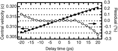
Figure 6. Linearity of the acceleration. The black squares show the velocity of the electron packet in dependence of the arrival time at the cavity relative to the microwave's phase. A linear fit (solid line) in the range of ±10 ps, covering the range of realistic arrival times of electrons from the photocathode, shows a good linearity. The residual is plotted in open circles. This measurement demonstrates the ability of the cavity to generate few-femtosecond pulses from much longer input pulses (see text).
Download figure:
Standard imageA variation of gv with the delay will lead to a shift of the temporal focus. Why is this critical? On the way from the cavity to a sample located at the temporal focus, the electron pulses compress linearly from the initial duration τdisp to almost zero. If the temporal focus shifts by a distance Δf, the pulse's duration increases by ∼τdispf/(f + Δf) at the sample. Assuming incoming pulses of τdisp = 500 fs, gv must not vary by more than 1% within the time window of τdisp in order to maintain compressed pulse durations of <5 fs at the sample. Changes of gv can originate from a varying frequency, from changes of field strengths in the cavity, or from nonlinearities within the time window during which the pulses can arrive. From our cavity's design, possible changes of frequency are <10−4. The power is stable to about ±0.1%, measured at the cavity's output port. The error in the linearity of the data shown in figure 6 is ∼0.36%. All values are low enough for achieving few-femtosecond duration at a fixed sample location.
10. Comparison of three different synchronization schemes
In the discussion of phase space in figure 2, jitter was neglected and pulse durations were defined with respect to the microwave's phase. In a practical pump–probe experiment, however, the effective resolution is limited by jitter between microwave and laser. Regardless of when exactly the laser impinges on the cathode, the electrons arrive at the sample at a time determined by the microwave's phase. For example, if the laser pulse arrives late with respect to the microwave's phase, electrons are also generated later. The cavity, however, accelerates them and they arrive at the temporal focus at the same time as electrons initially generated at other times. This is the intended effect of temporal compression in the cavity. However, the pump laser used for sample excitation is not affected by the microwave and the jitter therefore degrades the temporal resolution of the pump–probe experiments. Relative to the microwave's phase inside the cavity, the duration of the incoming pulses τtotal is determined by the duration of the laser pulses (τlaser), the effects of dispersion in the cathode–anode region (τdisp), and the jitter (τjitter). Assuming all distributions to be Gaussian, we obtain

The Wien filter provides a method of assessing the quality of synchronization, based on the principle of streaking in the longitudinal (energy) domain. The cavity maps the pulse duration τtotal into an energy spread ΔE = gEτtotal. For perfect synchronization, the measured ΔE would directly correspond to the electron pulse's duration at the cavity. In the presence of jitter, however, ΔE is larger. Measuring ΔE for different approaches for synchronization at otherwise unchanged settings therefore provides a relative comparison of which scheme delivers the lowest jitter. This is sufficient to improve the respective method, but not to determine the jitter's absolute value. However, an independent measurement or estimation of τlaser and τdisp can make the method more quantitative, as outlined below.
Figure 5 summarizes the results of such measurements for the three synchronization schemes described above. Figure 5(a) shows the central energy that the electron pulse obtains after the cavity, while scanning the phase. Figure 5(b) shows the energy spread for each phase delay, here for the case of synchronization with the 1209th-harmonic-PLL-VCO. At the compressing and anti-compressing phases at 0 and ∼80 ps, the energy spread is largest, because the cavity's time-dependent energy gain gE is highest. At ∼40 and ∼120 ps, no spread is induced, because the cavity only accelerates/decelerates the total packet without introducing significant dispersion. Note that energy spreads smaller than ∼20 eV are not reproducibly resolved with our Wien filter.
At the compressing phase, τtotal = ΔE/gE. The same holds for other phases with the respective gE there, because the pulse duration τtotal is <5 ps (including jitter), which is much shorter than the microwave's half-cycle (∼80 ps). We can therefore evaluate gE as the temporal derivative of the central energy (figure 5(a)) at each phase with exception of the maxima and minima. This improves the statistics and estimation of error compared to a measurement at the compressing phase only. Dividing the measured energy spread (figure 5(b)) by the corresponding gE provides the temporal spread τtotal at each point of the delay curve. These values should be constant.
Figure 5(c) shows the results. Plotted in squares are the values of τtotal obtained with the 1209th-harmonic-PLL-VCO, plotted in open circles are the results with the 76th-harmonic-PLL-VCO, and plotted as black dots are the values achieved with our direct extraction and amplification scheme. Clearly evident is a better performance of the two latter approaches, which give almost identical results despite their different conceptions. Considering the resolution of the Wien filter and statistical errors, we obtain τtotal = 3560 ± 100 fs for the 1209th-harmonic-PLL-VCO, τtotal = 715 ± 50 fs for the 76th-harmonic-PLL-VCO, and τtotal = 800 ± 150 fs for the direct extraction scheme.
11. Estimation of jitter
To assess the jitter quantitatively, we can use equation (2) and estimate the laser's pulse duration (τlaser) and the dispersive part of the incoming electron pulse's duration (τdisp). The laser pulses at the cathode had a duration of τlaser ≈ 70 ± 20 fs; this is the duration of the 266 nm pulses after a dispersive vacuum window. τdisp is determined by the photoemission bandwidth and the acceleration gradient [4, 17, 20, 33]. In our experiments, the photocathode was excited at a wavelength of 266 nm, corresponding to photon energies of 4.65 eV. The gold cathode's work function is Φ = 4.26 ± 0.1 eV [14, 34]. Assuming a half-spherical distribution of the photoemission, an initial energy spread between 0.2 and 0.3 eV can be estimated by measuring our source's divergence [14].
The acceleration field strength Eacc is given by the electrostatic potential and the distance between cathode and anode (the cavity in our case). For the three synchronization cases with the respective voltages and distances, we obtain acceleration gradients of 1.71 ± 0.06 kV mm−1 (1209th-harmonic-PLL-VCO), 2.11 ± 0.08 kV mm−1 (76th-harmonic-PLL-VCO) and 1.91 ± 0.08 kV mm−1 (direct extraction). The errors of these values are dominated by measurement errors of the cathode–anode distances (∼3%).
For calculating τdisp from an energy spread and an acceleration field, the literature offers several different models. The predictions of equation (2) in [20], equation (2) in [17], equation (1) in [33], equation (6) in [14] and equation (2) in [4] all scale with the same proportionalities, but have different pre-factors due to different assumptions about the electrons' initial velocity distribution. For example, an acceleration gradient of 2 kV mm−1 and an initial energy spread of 0.2 eV yields τdisp ≈ 750 fs [4], τdisp ≈ 520 fs [33] or τdisp ≈ 630 fs [14], respectively, depending on the model.
With the measured values for τtotal (see above), we can de-convolute τjitter according to equation (2) for the three synchronization cases, and for three models for the electrons' dispersion after photoemission, as explained above. Figure 7 shows the results for initial energy spreads of 0.2 and 0.3 eV. The upper and lower error bars are obtained by considering the experimental errors of τtotal and τlaser. In all cases, τjitter for the 1209th-harmonic-PLL-VCO lies between ∼3300 and ∼3600 fs, rendering this approach incapable of synchronization with femtosecond accuracy. In contrast, the two other approaches show τjitter in the range of ∼0–580 fs (76th-harmonic-PLL-VCO) and ∼0–770 fs (direct extraction), respectively, depending on the dispersion model and the initial energy spread.

Figure 7. Measured jitter for the 1209th-harmonic-PLL-VCO (circles), the 76th-harmonic-PLL-VCO (diamonds), and the direct extraction scheme (squares), calculated using different dispersion models. Model A is taken from [33], model B from [14] and model C from [4]. The left side was calculated for an energy spread of Δε = 0.2 eV, whereas the right side was calculated using Δε = 0.3 eV. A picosecond jitter is evident for the 1209th-harmonic-PLL-VCO, while the other two schemes show a jitter between zero and some hundreds of femtoseconds. A severe uncertainty arises from the choice of the dispersion model (see text).
Download figure:
Standard imageBy combining two cavities [21], the jitter was measured in the <100 fs regime with a very similar synchronization scheme as applied here, the 76th-harmonic-PLL-VCO [30]. This indicates that in our case the jitter is lower than measurable with our Wien filter. Limitations are given by three factors: firstly, the accuracy of the de-convolution of τjitter from τtotal is limited by the long duration of the dispersed electron pulses (∼600 fs in this work). Shorter durations of the pulses entering the cavity (below 100 fs) are possible by increasing the acceleration gradient and tuning the excitation wavelength closer to the work function of the photocathode [14]. This would strongly increase the accuracy of the de-convolution. Secondly, a large uncertainty originates from the choice of the appropriate model for calculating τdisp. A direct measurement of the initial angular and energy distribution of the electrons after photoemission, for example by time-of-flight-photoelectron emission microscopy (ToF-PEEM), would significantly improve the modeling of the dispersion. Modeling would be avoidable if the pulse duration before the cavity was measured, for example by ponderomotive deflection [35]. Thirdly, the energy resolution of the Wien filter limits the measurable τtotal. In the current setup, the large beam diameter, the achievable strength of the electrostatic and magnetic fields, and aberrations in the Wien filter are limiting the resolution. If all three aspects are improved, we expect that our approach will be capable of directly measuring synchronization jitter well below 100 fs. Even without an absolute assessment of jitter, the Wien filter provides a relative comparison between different synchronization approaches, and a direct experimental feedback for optimizations.
12. Conclusions
We may draw several conclusions from these results. Firstly, the Wien filter is a valuable diagnostic for operating a microwave cavity in the single-electron regime. It allows us to find the compressing phase, to measure the distance of the temporal focus, and to experimentally assess the relation between incoming power and effective acceleration gradient, including propagation effects. Secondly, the Wien filter provides information on the magnitude of laser–microwave jitter, at least relatively, as explained above. We can clearly distinguish between one not so good and two superior synchronization schemes. When optimizing the settings of the electronics, the Wien filter provides a direct and immediate feedback. It allowed us to identify the main contribution and origin of jitter in the 1209th-harmonic-PLL-VCO, which turned out to be thermal noise at one of the intermediate amplifiers. Thirdly, invoking models for the photocathode's energy spread, absolute values for jitter can be deduced. Two of the synchronization schemes show a jitter that is below the sensitivity of our measurement. The two concepts are quite different in nature and nevertheless show very similar upper limits of the jitter, making it probable that synchronization is actually better than reported here. Fourth, jitter analysis with an energy analyzer yields upper limits. This is conceptually different from other approaches, for example using two cavities [21], measuring feedback signals [30], or comparing in-loop with out-of-loop signals [36]. Such experiments may underestimate the real jitter, if systematical errors of the supposedly independent stages may cancel out. We emphasize here recent results on systematic amplitude-to-phase couplings and drifts in fast photodiodes [37, 38]. Such contributions to jitter may be hidden in the mentioned schemes, but are fully detected with our passive approach.
13. Outlook
The determination of values for jitter is not yet sufficiently accurate for our intention of reaching few-femtosecond resolution. The Wien filter's energy resolution is currently limited to ∼20 eV in our experiment. The next generation of an analyzer, based on ToF principles, is being constructed. Assuming τdisp = 100 fs [14] and a resolution of 2 eV, we should be able to characterize the jitter with an accuracy approaching tens of femtoseconds. The final proof of few-femtosecond pulse durations will require a measurement in the time domain. Ponderomotive scattering [35] or streak cameras [21] have a resolution of only ∼100 fs. A better possibility would be a direct interaction of optical fields and electron trajectories; such an experiment is currently attempted in our laboratories. The ability to produce a laser–electron cross-correlation with sensitivity on femtosecond scales will provide a feedback signal for the synchronization electronics that is sensitive to few-femtosecond changes. This will decrease the jitter accordingly.
A microwave cavity can also be applied to highly coherent, but temporally long electron sources, for example from atomic condensates [39–40]. As explained with figure 2, longer initial pulses could still be useful for reaching few-femtosecond duration after the cavity, if the initial energy spread is low enough. An advantage would be higher coherence and better ability to focus, but a disadvantage would be a very long distance of the temporal focus, if excessive energy spreads shall be avoided. In conventional electron microscopes, coherence is increased by filtering in condenser units, after which one electron at a time is emitted. In a time-resolved microscope, space charge in the path before the filters increases the pulse duration. A microwave cavity, however, could compensate this and provide single-electron pulses of sufficient coherence for direct imaging in microscopy. In all of these cases, analysis of the output energy and spread, as developed here, will provide valuable data about mechanisms and performances.
Acknowledgments
This work was supported by the Rudolf-Kaiser-Stiftung, the Munich-Centre for Advanced Photonics, the European Research Council (Grant '4D imaging') and the International Max Planck Research School of Advanced Photon Science. The authors thank Ernst Fill for helpful discussions at the initial stages of this research and Grigori Kurkin, Vladimir Tarnetsky and Igor Zapryagaev for their help with setting up some of the synchronization electronics.