


Abstract
We show that the presence of an interaction in the quantum walk of two atoms leads to the formation of a stable compound, a molecular state. The wave function of the molecule decays exponentially in the relative position of the two atoms; hence it constitutes a true bound state. Furthermore, for a certain class of interactions, we develop an effective theory and find that the dynamics of the molecule is described by a quantum walk in its own right. We propose a setup for the experimental realization as well as sketch the possibility to observe quasi-particle effects in quantum many-body systems.
Export citation and abstract BibTeX RIS
GENERAL SCIENTIFIC SUMMARY Introduction and background. Quantum walks represent the quantum motion of a particle on a lattice with a strictly local dynamics, meaning that in a finite time the walker propagates over only a finite distance. This situation can be realized with spinor particles by applying an alternating sequence of spin-dependent shift operations and coherent spin manipulations. The fully discrete nature of such quantum systems—both in space and time—makes them highly attractive in a wide range of quantum applications, e.g., from their utilization as primitives for quantum information processing to the possibility of simulating complex quantum-mechanical systems. As a first step in this direction, we study here the problem of two interacting walkers forming molecular states.
Main results. We analytically predict that on-site interactions in a two-particle quantum walk give rise to a dynamically stable bound state. Proving that the distance between the two particles is exponentially bounded, we interpret these bound states as molecules and develop an effective theory that describes their dynamics as the quantum walk of a single compound particle (see the figure). We make an experimental proposal based on realistic conditions to test the prediction of molecules using individual atoms in optical lattices.
Wider implications. Our result is a first important step in a bottom-up approach towards the simulation of collective excitations of many particles, e.g., Cooper pairs or excitons. In addition, the discrete nature of our system could open new routes for controlling and studying decoherence and damping in simulated quantum systems.
 Figure. Joint distribution of the positions (x1 and x2) of two spin-1/2 particles on the line undergoing a two-particle Hadamard quantum walk without (left) and with (right) interaction. The peak around the diagonal (x1 = x2) indicates the formation of a combined molecular state.
1. Introduction
Bound states play a central role in nature, and their significance cannot be overstated, as they are the basis of the existence of any kind of structured matter. Molecules, for instance, are compounds of atoms which, due to Coulomb interaction, remain bound together and move as a single-quantum particle. The particular properties of molecular states depend on their interaction potential, which typically can form a covalent, ionic or van der Waals bond; very diverse in their character, the so-called halo dimer states consist of weakly bound pairs with the wave function extending far out of the classically allowed range [1]. These states have been long studied and observed in different physical systems, from the investigation of light atomic nuclei [2] to atomic [3] and molecular systems [4, 5].
In this work, we predict and study a novel class of molecular bound states appearing in systems moving under the influence of a periodic driving force. In the spirit of Floquet theory, the system's dynamics can be regarded as discrete in time, i.e. each evolution step takes one period τ in real time. The spatial coordinate is likewise confined to a periodic lattice. Since, in addition, particles can move only by a strictly finite distance in each step, we are dealing with so-called quantum walks. The molecule-forming interactions occur through on-site contact potentials. Quantum walks of non-interacting particles are currently under investigation in many groups.
Even such free walks, employed in a search algorithm, promise dramatic speedups relative to algorithms based on classical random walks [6, 7]. The interaction that we introduce between the walking quantum particles adds a decisive new element, an entangling quantum gate, which is essential for further non-trivial computational tasks and ultimately for universal quantum computation [8]. Much simpler than universal computation, but still a challenging goal, is the construction of a discrete quantum simulator for quantum lattice systems based, e.g. on interacting neutral atoms in an optical lattice. A quantum simulator would be helpful, in particular, for understanding the formation and dynamics of quasi-particles such as Cooper pairs or excitons. In this direction, the study of molecules is the first important step in a bottom-up approach to collective excitations, in which the formation of compounds can be analyzed in full detail, before many particle effects such as background-induced decoherence and damping set in.
Many of the theoretical tools for studying the formation of bound states are analogous between discrete-time and continuous-time systems. For example, the relation between 'free' and 'interacting' dynamics is governed by a scattering theory, in which bound states appear as poles in the S-matrix. Other intuitions must be modified, most notably the notion of 'binding energy'. In continuous time and space, the binding energy, i.e. the energy of a compound below the continuum, is directly relevant to the stability of the compound. However, in discrete time, the distinction between high and low energies and, accordingly, between repulsive and attractive interactions is lost: just like momentum in a lattice becomes quasi-momentum, which is defined only up to multiples of 2πℏ/a with a the lattice constant, according to the Floquet theory [9] energy becomes quasi-energy, which is defined only up to multiples of 2πℏ/τ. Therefore, our criterion for molecular binding will not be in terms of the spectrum of the time evolution operator, but dynamical: we define a molecular state of two atoms as one in which the distance between the constituents remains bounded for all times, even though the center of mass degree of freedom exhibits quantum spreading of wave packets. This dynamical stability distinguishes molecules sharply from quantum correlations recently reported for the quantum walk of non-interacting photons, which are due to a Hong–Ou–Mandel-like two-particle interference effect [10–12]. In such systems the constituents will always move apart for large times. Moreover, in contrast to the Hong–Ou–Mandel effect, our molecular binding mechanism is quite independent of Bose/Fermi symmetrization, since it can equally be demonstrated between atoms of different species.
Quantum walks have recently been demonstrated experimentally in a variety of setups [13–19]. While all these experiments show the expected one-particle dynamics, their ability to demonstrate the type of interaction we describe differs very much. In the optical lattice implementation [13] interactions are very natural if not unavoidable: when two atoms sit in the same potential well of an optical lattice they are expected to pick up a collisional phase depending on the duration of the contact. Free atom evolution in these systems is realized by simply coupling two internal atomic states by microwave fields and shifting the positions according to their internal states. Under these conditions we predict the formation of stable compounds of two atoms, which move according to a quantum walk in their own right.
The relevant conditions and parameters for an implementation of molecules of two atoms walking in a one-dimensional (1D) optical lattice are discussed below. Our conclusion is that an experiment should be possible in the near future, perhaps even by extending an existing experimental setup. On the theoretical side, our work was partly inspired by analogous work in the continuous-time case [20]. A correlation effect due to molecular binding was seen in a numerical study [21], albeit without explanation.
When this work was finalized we became aware of similar results reported by Lahini et al for the case of two interacting Bose particles [22].
2. The system
We have chosen a simple standard system for which all details of molecular binding can be demonstrated explicitly. The free evolution of the constituents is realized by the well-known Hadamard walk, and we consider an interaction depending on a single parameter. The molecular binding phenomenon occurs in a much broader context, which is demonstrated by the analysis in section 5. However, for definiteness and ease of presentation, we will stick until then to the model system that we will now describe.
The particles move on the lattice of integer positions, where we take the lattice spacing a = 1 without loss of generality, and have an additional two-level internal degree of freedom. Hence, for a single particle the basis states are |x,α〉 with an integer x labeling the positions and α = ± labeling two orthogonal internal states. The unitary walk operator W1 of a single particle is composed of two operations,  , namely a state-dependent shift

and a coin operation, which apply a 2 × 2-matrix H to the internal degree of freedom. For this, we choose the Hadamard matrix

With this choice, we follow the most widespread convention, although from the point of view of experimental implementation it would be more natural to take instead the matrix of rotation by the angle π/4.
The walk of two non-interacting particles is now just given by the tensor product W2 = W1⊗W1. The basis vectors of such a two-particle system are hence |x1,α1,x2,α2〉. The interaction is given by an additional phase factor, which is applied only on the collision subspace spanned by the basis vectors with x1 = x2. The corresponding unitary operator G is thus given by

The collision phase g is the only free parameter in this model. The overall walk is W = W2G.
It will be useful in the following to identify the discrete symmetries of the walk. If we then choose the initial state in an invariant subspace of a symmetry operator we can simplify the problem by restricting all operators to this subspace. The first symmetry arises from the observation that the shift S changes x by ±1 in every step. Since the coin operations and G do not act on position, the parity of the relative coordinate x1 − x2 is invariant, i.e. the walk preserves checkerboard color. In order to let the two particles interact, we will always choose an initial state with x1 − x2 even, since the interaction G is otherwise the identity in the odd subspace.
The second discrete symmetry is related to the center-of-mass coordinate (x1 + x2)/2, and it arises from the translational invariance of the system under joint shift of both coordinates by an integer number of steps. The invariant subspace associated with this symmetry is constituted by the states of given center-of-mass momentum, which is a conserved quantity under the walk W; in section 3.2, this discrete symmetry is discussed in greater detail and used to derive the energy spectrum of the system. The broken Galilean symmetry has important implications for the properties of molecules, which will eventually be a function of the center-of-mass momentum.
The third symmetry originates from the invariance of the system under time translations by an integer number of intervals τ, where we can set τ = 1 without loss of generality. While continuous-time translational symmetry implies conservation of energy, in our system where the walk operator W is periodically applied the energy is conserved up to integer multiples of 2π.
Finally, the fourth discrete symmetry of the system is the exchange of the two particles. The symmetric and antisymmetric subspaces are therefore invariant. We will only consider the dynamics in the antisymmetric subspace, because this turns out to be slightly simpler. The reason is that upon collision, say for x1 = x2 = x, the combination of internal states |α1,α2〉 must be the singlet state  . The standard initial state will be with both particles at the origin, so Ψ = |0,0〉⊗ψ−.
We note that the proposed experiment runs with bosons. There are nevertheless two ways to realize the above system. The first uses a slightly different interaction G, which also suppresses the action of the Hadamard coin on the collision subspace. Then, assuming that particles start from different sites, the only way they can come to the same site x is by shifting them from the neighboring lattice sites, x ± 1. Then the internal state at collision points is always  , and exactly the same analysis as in the Fermi case applies, with ψ+ replacing ψ−. The second possibility is to use further states of the system, such as vibrational ones, to prepare the initial state with the required fermionic symmetry under exchange of particles. It is worth underlining in this context that the molecular binding effect we describe does not depend on the indistinguishability of the particles. The same could be done with atoms of different species, provided they can be trapped in the same optical lattice.
3. Identifying the molecules
3.1. Simulation in position space
The easiest way to see the molecular binding effect is by direct simulation of the dynamics described in the previous section, starting from the standard initial state (internal singlet at the origin). The resulting joint probability distribution of the positions (x1,x2) after t = 50 steps is shown in figure 1, which allows a direct comparison between the non-interacting case g = 0 and the maximal interaction phase g = π. Both pictures are symmetric with respect to the main diagonal x1 = x2. In the non-interacting case, the dominant features are two peaks at x1 = −x2 with  . These peaks are well known from the Hadamard walk of a single particle, and to facilitate the comparison, a dashed square with sides at
  is shown in the left panel. There is a correlation effect resulting from the antisymmetric initial state [10], which is expressed by the absence of peaks at
  .
.
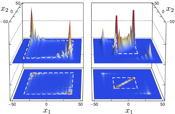
Figure 1. Joint probability distribution of two particles after t = 50 steps of an interacting Hadamard walk with antisymmetric initial state. Left panel: without interaction (g = 0); right panel: interaction with collisional phase g = π. The embedded squares are for comparison with the theoretically calculated peak velocity of the free Hadamard walk (left) and the peak velocity of the effective walk of the molecule (right).
Download figure:
Standard imageTurning to the interacting case we observe the following main features:
- (a)The peaks near
 are still visible, but smaller. Indeed, they will continue to move as in the non-interacting case because particle pairs with a long distance do not see the interaction anyway. It will be shown later in section 3.6 that the total weight of these 'free' peaks is 1/3.
 - (b)The rest of the probability is concentrated near the diagonal x1 = x2. Along the diagonal the spreading is proportional to the time, which is called ballistic behavior in the context of quantum walks. The center-of-mass motion of the molecules thus exhibits the same behavior as other walking particles, including two leading peaks. These are slower than the single-atom peaks. We will later show them to be at x1 = x2 = ± t/3 for large number of steps t.
- (c)The width around the diagonal is constant in time. More precisely, apart from the free peaks that move away, the probability to find |x1 − x2| > r decreases exponentially in r, with constants independent of t. This is the dynamical statement of molecular binding.
3.2. Numerical determination of the quasi-energy spectrum
Another signature of molecular binding can be identified in the eigenvalue spectrum of the walk operator W. Since, by construction, it commutes with the joint translations (x1,x2)↦(x1 + a,x2 + a) we will jointly diagonalize the walk operator W with the unitary translation operator T. Both operators are unitary and hence have eigenvalues on the unit circle. For graphical representation we unwrap these circles and hence represent a pair of eigenvalues  of T and W by a point (p,ω) in the square [ − π,π] × [ − π,π]. This introduction of quasi-momentum p in the Brillouin zone [ − π,π] is very familiar from solid state theory. Here, as generally in discrete time dynamics and Floquet theory, we do the same for the quasi-energy ω.
In order to obtain the joint eigenvalues numerically we close the system to a ring of length L. The resulting Hilbert space will have dimension 4L2, so the diagonalization can be carried out numerically for fairly large ring sizes. A typical result (again with interaction phase g = π, and for a small ring size L = 32) is shown in the right panel of figure 2.
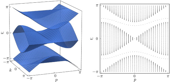
Figure 2. Spectrum of the interacting walk operator for two particles on a ring with 32 sites. Left panel: in the non-interacting case relative momentum is also conserved and is represented as a third direction, orthogonal to the paper plane. For large rings the points fill the blue surfaces. Right panel: in the interacting case (g = π) the bands are equal to the projection of the left-panel figure onto the (p,ω)-plane. The additional feature introduced by interaction is the chain of simple eigenvalues in the band gap, i.e. the molecule states.
Download figure:
Standard imageThe densely filled regions, which we call bands, can be understood completely from the non-interacting case. To this end consider the left panel in figure 2. The free walk operator commutes not only with joint translations but also with separate translations of the particles. Therefore, we can jointly diagonalize the two separate translation operators and the walk operator, resulting in a cube with axes total quasi-momentum p = p1 + p2, relative quasi-momentum k = (p1 − p2)/2 and quasi-energy ω, respectively. In the figure, k is taken as depth, roughly perpendicular to the paper plane. Now, from the known spectrum of the single-particle walk W1 we can immediately determine the joint spectrum of W2 explicitly. This gives the blue surface in the left panel. The points on that surface are the discrete eigenvalue triples (p,k,ω) one obtains by closing the system to a ring of the same size as in the right panel. Consider now the image obtained by a parallel projection of the left panel figure to the paper plane: this gives the bands also observed in the interacting case. To be precise, for finite L the continuum eigenvalues do not fall exactly on the interacting ones inside the bands: there is a slight deformation due to the interaction. However, as we will show in section 5, the continuous spectrum obtained in the limit L → ∞ is independent of the interaction phase g.
The new features due to the interaction are the lines of eigenvalues appearing in the gaps between the bands (see the left panel). These are the molecular bound states that will be determined analytically in the following section.
3.3. Analytic solution of the Schrödinger equation for bound states
We will only sketch the main ideas, because the derivation will be given with more detail and in a much more general setting in section 5.
For two-particle systems with continuous translational symmetry, and an interaction depending only on the distance of the particles, the obvious first step for identifying molecular states is to introduce center-of-mass and relative coordinates. The same is true in the lattice case, but with an important difference: in continuous space the decoupling is complete, and the problem to be solved for the relative motion is not only independent of the center-of-mass position but, by Galilean boost invariance also independent of the total momentum. In discrete space, this symmetry is meaningless and the relative motion in general depends on the total quasi-momentum p = p1 + p2. In the momentum representation, this means that the diagonalization of W can be done separately for each value of the conserved quantity p, and one is left with a problem in a space of wave functions depending on the relative momentum k = (p1 − p2)/2, with p treated as a fixed parameter. The ranges of p and k can be taken to be [ − π,π] by a suitable reshuffling of Brillouin zones (see section 5.1).
The free walk thus leads to the operator

acting on the tensor product of the two internal state spaces. The collision space is given by (x1 − x2) = 0, which in the momentum representation corresponds to the constant functions of k. We denote by N the projection onto this subspace, so  . Then

and Ψ is an eigenvector of W = W2G with eigenvalue exp(iω) if

One can show by a transfer matrix argument that in the case at hand there are no eigenvalues embedded in the continuous spectrum. Therefore, from now on exp(iω) is understood to be in the spectral gap of Wp, i.e. Wp(k) − exp(iω) is invertible for all k. According to our choice of the antisymmetric subspace in section 2, NΨ must be proportional to the singlet ψ−, and we can choose NΨ = ψ−. We can thus solve (6) for Ψ:

What determines the eigenvalues ω is the consistency condition NΨ = ψ−. This means that we have to evaluate the integral over k of the right-hand side of (7). Since Wp depends on k as a polynomial in  , this integral is a complex integral over the unit circle, which can be evaluated via the residue theorem. The resulting equation can be solved, and gives


Condition (9) results from picking only poles inside the unit circle for residue evaluation. The two branches of relation (8) are plotted in figure 3, and directly confirm the numerical result in figure 2. Some of the eigenvalue curves end at the edge of the continuous spectrum, because (9) has to be taken into account. Ignoring that condition leads to unphysical 'virtual' molecule states, shown in the right panel of figure 3.
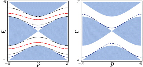
Figure 3. Left panel: quasi-energy spectrum as a function of the total quasi-momentum p. Dispersion relations ω(p) of molecular bound states (lines, with g = π/4,π/2,π,3π/2 from bottom to top), continuum of free particles (shaded area). Right panel: quasi-energy spectrum for interaction phase g = π/4 including the virtual bands (dashed), which satisfy (8) but not (9).
Download figure:
Standard imageOf course, for admissible triples (g,p,ω), (7) gives an explicit expression for the bound state wave function. These functions or rather their Fourier transforms from the variable k to the variable (x1 − x2) are shown in figure 4 for two values of g. Clearly, they are decaying exponentially on the scale of a few lattice sites. See section 5.4 for a explicit construction of the eigenfunctions.

Figure 4. Eigenfunctions (absolute value squared) of the relative motion as a function of p (white lines), after (20). The surface arises by analytically interpolating to non-integer values of x1 − x2. Left panel: g = π/4, both branches shown in figure 3. Right panel: g = π either branch.
Download figure:
Standard image3.4. Effective molecule dynamics
Let us now turn to the dynamical characteristics of the molecules. Choosing, for each p, normalized eigenfunctions χ±p(k) in the upper and in the lower gap wherever they exist, we can write the overall wave function of a molecule as Ψ(p,k) = ϕ+(p)χ+p(k) + ϕ−(p)χ−p(k). Here, it is understood that we put ϕ±(p) = 0, whenever the corresponding branch is ruled out by (9). The time evolution of such wave functions will be completely determined by the branches ω±(p) of the quasi-energy. After t time steps we get

The factors χ just play the role of a 'spinor basis' for the space of internal states of the molecules. With this abstraction we have a discrete time evolution Weff on a lattice, with two internal degrees of freedom, although some internal states may be forbidden for some values of p. This is the effective time evolution of the molecules.
However, it is far from clear whether Weff is again a quantum walk, i.e. whether it allows for a description in position space that involves only strictly finite jumps. The position representation of an effective walk is obtained from the momentum representation by Fourier transform which can, however, be preceded by a p-dependent basis change. Up to such a change the walk is obviously given completely in terms of the dispersion relations ω±(p). Hence, the question boils down to deciding whether these functions are the dispersion relations of some quantum walk. Since the full interacting walk has strictly finite jumps for pairs of particles, it would seem natural that the subspace of molecule states inherits this property. However, the projection to the molecule subspace (given by the eigenfunctions χ±) is not local, since the eigenfunctions are only exponentially localized.
It turns out that for the family of interacting Hadamard walks studied here Weff is indeed a quantum walk. This family even allows for a simple decomposition into a single shift and coin operation:  with the shift (1) and a 2 × 2 coin matrix C. Indeed, we exactly obtain the dispersion relations (8) with the coin

The walk uses both branches in (8), though only 'virtually' if one or both of them are forbidden by the constraint.
The asymptotic position distribution of Weff can be computed directly from the dispersion relation ω±(p). In fact, for any walk the probability distribution of Q(t)/t, i.e. the position in 'ballistic scaling', converges to the distribution of the group velocity operator V [23]. V has the same p-dependent eigenvectors as W, but eigenvalues ω±'(p) = dω±(p)/dp instead of  . Thus, we can compute the asymptotic position distribution directly for every initial state, and this depends only on the joint distribution of p and the branch index ±. For an initial state at the origin the quasi-momentum distribution is flat. Therefore, when ω± has an inflection point at some p*, the group velocity ω±'(p*) has a maximum, and consequently the probability density has a square root singularity ('caustic'). This explains all the peaks seen in the simulated position density diagrams of this paper. For the free Hadamard walk, the peaks are at
  . For the effective walks with coin (11) the inflection point is always at p* = ± π/2 (see figure 3). The left panel of figure 5 shows the asymptotic velocity distributions as a function of the interaction parameter g. For g < π/3 and g > 2π − π/3, the constraint (9) forbids momenta around p*. Hence, the quasi-momenta producing the caustic peaks in the effective walk starting from the origin fall into the virtual branch of the dispersion relation, and have probability density zero. Hence, we expect not to see any peaks in the walk of molecules. This is confirmed by the right panel in figure 5, and the corresponding asymptotic distribution (blue line) in the right panel.

Figure 5. Left panel: molecule's asymptotic position distribution in ballistic scaling, i.e. the probability density for group velocity ω'(p), as a function of the interaction parameter g. Highlighted are the cases g = π/4 (continuous) and g = π (dot-dashed). The vertical scale is limited to the [0,1] interval. Right panel: position distribution of an interacting Hadamard walk with interaction phase g = π/4, after 50 time steps. The flat distribution of the molecule state corresponds to the absence of caustic peaks in the asymptotic position distribution.
Download figure:
Standard image3.5. Bloch oscillations
The single-particle character of the molecular state can also be seen from its reaction to an additional static force. Such a force can be modeled by an additional position-dependent phase factor that the particles acquire in each time step. This results in additional shifts in the total momentum variable, and is seen as an oscillation of the molecule's position distribution. Such oscillations occurring at a frequency proportional to the gradient of the external potential are well known as Bloch oscillations in condensed matter physics [24]. As can be seen in figure 6 the oscillation of the bound state exhibits a doubled frequency, i.e. the molecule experiences twice the force as compared to the single particles. Bloch oscillations lead to rapid dissociation of the molecule, if they can shift momentum to a region without bound state, e.g. g = π/4 in figure 3. Even for the most stable case g = π, however, the static force will eventually dissociate the molecule, which is foreshadowed by the slow increase of the variance in figure 6.
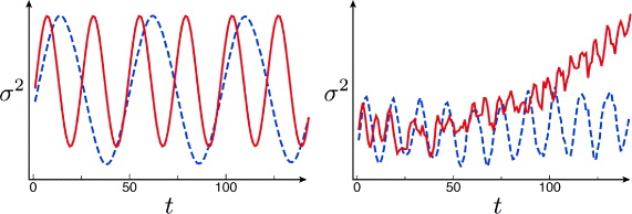
Figure 6. Bloch oscillations of the variance (σ2) of the position distribution for the molecule (solid) and single particles (dashed) with interaction phase g = π. In every time step, a phase of xπ/48 (left panel) or xπ/14 (right panel) is applied at position x reproducing the effect of a static force. The double oscillation frequency for the molecular state indicates a two-atom bound state. After t = 100 time steps around 3% (left) and 25% (right) of the molecule are dissociated into free particle states. Vertical axis in rescaled units.
Download figure:
Standard image3.6. Preparation probability
Molecules have to be initially prepared. In order to make them detectable in an actual experiment, their preparation efficiency has to be sufficiently high. Since the dynamics of the walk W itself has no dissipation, an initial state with two widely separated atoms would have negligible overlap with any bound state, and this remains true for all times. However, by initially using a dynamics that is different than W it is possible to prepare two atoms in the same site (see section 4). This state then has a non-zero overlap with molecule states. The resulting probability of forming a molecule, i.e. the modulus squared of the overlap, will be studied in this section showing its dependence on the interaction parameter g.
Starting from two atoms in the same lattice site, the formation of molecule states is apparent from figure 1: by just letting the interacting walk run for a few steps the unbound pairs will move away, and the remainder is in the molecular state. The critical parameter for this second stage of the preparation is the modulus squared of the overlap of the initial state with the molecular subspace Povl(g).
As before, the computation of Povl(g) is done separately for every quasi-momentum p and every branch ω± of the dispersion relation. The result Povl(p,g) is plotted in figure 7. Since we consider the situation of a localized initial state, Povl(g) can be determined from Povl(p,g) by integration over p. This integrated overlap (see right panel in figure 7) has a maximum at g = π; so this case, also shown in figure 1, has the highest preparation efficiency Povl(π) = 2/3.

Figure 7. The figure shows the modulus squared of the overlap Povl(p,g) for the ω+ branch (left graph), the sum of both branches (right graph). On the side of the right graph the integrated capture overlap Povl(g) is shown.
Download figure:
Standard image4. Experimental proposal
We plan to realize walking molecules by extending an existing experiment [13], where discrete quantum walks are realized with single neutral Cs atoms in optical lattice potentials.
In these systems, the natural choice for implementing the spin degree of freedom consists in choosing two long-living internal states of the hyperfine ground state S1/2, namely | − 〉 = |F = 3,mF = 3〉 and | + 〉 = |F = 4,mF = 4〉.
The coin operator (2) that couples these two states is realized by resonant microwave fields oscillating at the atomic clock frequency near 9.2 GHz; Hadamard-like coin operators, such as σzH with σz the Pauli matrix, are simply obtained by applying π/2 resonant microwave pulses in a time τcoin of about 10 μs. A fidelity of 99% per coin operation has been experimentally attained [25].
The spin-dependent shift operations (1) are implemented by working with the so-called spin-dependent optical lattices, which exhibit large vectorial polarizability [26]. The basic principle is shown in figure 8(a), where atoms are subject to a laser beam tuned to a frequency ωL = (2/3) ωD2 + (1/3) ωD1, with ωD1 and ωD2 being the frequencies of fine structure doublet of Cs atoms; this corresponds to a wavelength λL = 2π/ωL = 866 nm. In this case they experience a dynamical polarizability which, depending on the spin state, is sensitive to either one of the two circular polarizations. By working with counterpropagating waves in the lin–θ–lin configuration, the ac-Stark shift yields two independent optical lattice potentials, both characterized by a lattice constant a = λL/2, but associated respectively, with σ+ and σ− photons, where their relative position is controlled by rotating the polarization angle θ as shown in figure 8(b). Since in deep optical lattice potentials site-to-site tunneling is perfectly negligible, atom positions follow the displacement of the spin-dependent potential in which they are trapped; for example, a π rotation produces a shift of exactly one lattice site [27–30].
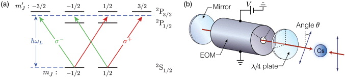
Figure 8. Spin-dependent shift operations in optical lattice potentials. (a) Allowed optical transitions by circularly polarized photons σ+/− are shown in fine structure; with the lattice laser frequency ωL in between the D1 and D2 lines, the ac-Stark shift cancels for the dashed transitions. As | ± 〉 shares mostly mJ = ± 1/2 character, these two states experience light shift from complementary circular polarizations. (b) The linear polarization of the counterpropagating wave is rotated by an angle θ determined by the voltage V , which is applied to the electro-optic modulator (EOM). The periodic polarization gradient experienced by Cs atoms yields two optical lattices, one for each of the coin states | ± 〉, with θ setting the relative distance.
Download figure:
Standard imageIn order to reduce spurious motional excitations below 1% level, the transport time is adjusted to be a multiple of the oscillation period of the atomic motion along the lattice axis [31]; typical transport times τshift are about 20 μs.
Decoherence due to inhomogeneous dephasing of spin states, produced, for instance, by stray magnetic fields, is mitigated by repeatedly applying spin-echo π pulses at each walk step; this allows coherence times T☆2 ≈ 1 ms, making several coherent walks W1 feasible in this lapse of time.
The use of ultracold collisions in spin-dependent optical lattices was first proposed by Jaksch et al [27] as a mechanism to generate entangled states of several atoms. We propose to use here the same on-site interactions via s-wave cold collisions in order to acquire the phase shift for the formation of molecules. In the first proposal interactions were considered through a perturbative approach, which was later extended to account for trap-induced resonances through pseudopotential methods [32–35]. This second route has the merit of making reliable predictions even for interaction strengths beyond the perturbative limit, thus allowing us to treat considerably faster collision rates. The physical assumption here is that the atomic interaction potential is not modified by the presence of the external confinement, which imposes  with r0 the van der Waals interaction range, μ the reduced mass, and ω the trap frequency; this constraint satisfies automatically the other implied condition that scattering occurs only by s-wave collisions. In this way, all the parameters of the interaction pseudopotential depend only on the free-space (energy-dependent) s-wave scattering length.
The use of Cs atoms is especially favorable because the large triplet scattering length of the electronic ground state aT ≈ 2400 a0 allows strong interactions leading to fast phase accumulation [36]; in this case, the van der Waals interaction range is equal to r0 ≈ 5 nm, limiting the trapping frequency to ω ≪ 2π × 5 MHz. Roughly, given a 3D optical lattice with isotropic harmonic confinement ω = 2π × 30 kHz, the triplet state  acquires a collisional phase shift g = π in about 10 μs. This is just below the current step time of our experiment τ = τshift + τcoin, so that it could be well incorporated. Stock et al [35] also studied losses induced by inelastic scattering due to spin–spin and and higher-order spin–motion coupling, and they found that losses are negligible at energies smaller than 5 μK.
The probability to produce a molecule starting from two atoms initialized in the same lattice site in the spin state |ψT〉 has been computed in the previous section (3.6) and is equal to 2/3 at g = π. This initial state can be easily obtained from two atoms that are first loaded at different sites in opposite spin states and then displaced to the same site through spin-dependent transport operations [30, 37]. Molecules will be detected by analyzing the position correlations of the two atoms, seeking the diagonal feature shown in figure 1(b). An optical resolution of the imaging system capable of resolving single lattice sites is required in this experiment, and it can be obtained by numerical analysis of fluorescence images which are recorded by a high-resolution microscope [38–40].
As the collisional phase depends on the motional state of trapped atoms, in order to make interactions precisely controlled and coherent it is necessary to initialize atoms in the motional ground state. Ground state cooling along the lattice axis is routinely achieved in the present setup [41], while atoms still occupy several motional states in the lateral direction where the confinement is much weaker. Cooling in the radial direction can be achieved as well, for instance, by Raman sideband cooling once the lateral confinement has been enhanced to the Lamb–Dicke regime [42]; alternatively, atoms could be prepared in the motional ground state starting from a Mott insulator state. Obtaining average vibrational quantum numbers 〈n〉 < 5 × 10⁻³ in all three directions is well expected, thus allowing sufficiently many coherent steps to clearly demonstrate the molecular binding effect.
Atomic systems not only offer a natural way to implement on-site collisions but also promise great flexibility in engineering interaction operators G. For instance, for bosonic particles as 133Cs atoms, triplet spin states permit implemention of interaction operators acting on a 3D collision subspace. The simplest case is the one in which the collision subspace is reduced to one dimension: collisions between Bose particles resemble those of Fermi particles, since the interaction operator G in (3) contributes only with a phase factor. This situation can be realized by exploiting the interaction-induced level shift of |ψT〉, which can render the coin operations at 9.2 GHz ineffective at collision points in the case the scattering lengths for the three pairs of states are different, a↑↑ ≠ a↑↓ ≠ a↓↓. This has the effect of suppressing the transitions to | + +〉, | − −〉 because of interaction blockade [43], thus effectively restricting the collision subspace to a single dimension.
Furthermore, the possibility of associating an additional quantum label with each particle, for instance, the number of the occupied motional state, allows different classes of molecules—Fermi, Bose or distinguishable particles—to be studied depending on the symmetry of the initial state. For instance, Fermi-like molecules can be obtained with bosonic Cs atoms by starting from a singlet state  , which can be prepared by a simple spin rotation of only one particle applied to an entangled state like the one produced by Mandel et al [44]. Spin states with S = 0 exhibit the correct fermionic behavior under particle exchange, and, being rotationally invariant, they are also preserved during both s-wave collisions and free-particle walks.
5. Theoretical analysis
In this section, we show how the theory works starting from a general translationally invariant walk: not necessarily nearest neighbor, in any lattice dimension and with arbitrary coin dimension. The interaction will still be only at a collision point (x1 = x2), but this does cover any finite range interaction by grouping cells to supercells.
The first subsection gives a more careful discussion of the introduction of center of mass and relative coordinates, and the implicit reorganization of Brillouin zones needed. In the second we develop the general theory of point perturbations of quantum walks, which can then be applied to the relative motion as described above. In order to prove that every point in the gap can be a quasi-energy for some bound state we need a lemma, that we prove in the third subsection. Finally, we derive the form of the bound state wave functions, and apply this to the interacting Hadamard walk.
5.1. Relative coordinates
Here, we will give a short account of the introduction of relative coordinates in a two-particle quantum walk. We will look at a slightly more general setting allowing the walkers to move on an s-dimensional lattice and carrying a d-dimensional internal state.
In analogy to section 2, we can then pass via Fourier transform from the tensor product of the two particles position and internal states in the Hilbert space  to the quasi-momentum representation in
 ![$L^2([-\pi ,\pi ]^2,\mathrm {d}p_1 \mathrm {d}p_2)\otimes {{\mathbb C}}^{2d}$](https://content.cld.iop.org/journals/1367-2630/14/7/073050/revision1/nj426440ieqn18.gif) . This corresponds to a change of variables from the lattice positions x1, x2 of the two particles to their quasi-momenta p1, p2.
. This corresponds to a change of variables from the lattice positions x1, x2 of the two particles to their quasi-momenta p1, p2.
The generator of joint particle translations is the total quasi-momentum p = p1 + p2, which hence commutes with the walk. The remaining variable is the relative quasi-momentum k = (p1 − p2)/2. The factor 1/2 in the definition of k allows us to define the first Brillouin zone again as [ − π,π]2. Figure 9 shows how this is done by identifying points outside [ − π,π]2 with points inside this interval in the 1D lattice case (or separately for every component of the quasi-momentum vector in higher dimensions).
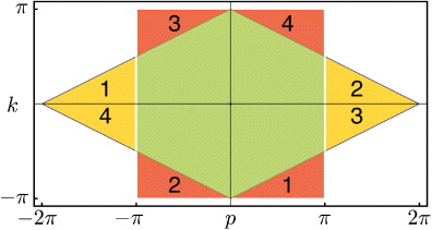
Figure 9. Domains for the variables p1,p2 and p = p1 + p2,k = (p1 − p2)/2, and the reorganization of Brillouin zones required to make both sets of variables run over [ − π,π]2.
Download figure:
Standard image5.2. Point perturbations
The core of the computation in section 3.3 was done in relative coordinates, and effectively reduced to studying a quantum walk perturbed at the origin. This problem is also of independent interest, and we will here treat such systems in generality. We allow a lattice of arbitrary dimension s, i.e.  . The Hilbert space of the walk is then
  for some finite-dimensional internal space
  . The 'free' evolution will be an arbitrary unitary operator W0 commuting with translations. By Fourier transform we pass to the momentum representation, so
  is seen as the space of square integrable functions Ψ(k) on the Brillouin zone [ − π,π]s with values in
  . In this representation W0 thus acts by multiplication with k-dependent unitary matrix W(k).
We usually take it as part of the definition of a quantum walk that W0 has a strictly finite propagation region. In this case each entry of the corresponding matrix W(k) is given by a trigonometric polynomial, i.e. a finite linear combination of functions  with n a vector with integer components. We will not use much of this structure, but only that the eigenvalues
  of W(k) can be taken as a set of differentiable functions in the neighborhood of almost every k.
The subspace of  of functions, which are non-zero only at the origin, becomes in momentum space the space of k-independent functions. The corresponding projection N is

Here, we have indicated that we denote by NΨ both the constant function in  and its value in
  . By modifying the unitary operator W0 exactly on this subspace by a unitary operator Γ acting on
  we get the perturbed walk as

Note that as long as Γ is unitary, the second factor on the right-hand side of (13) and therefore also W have the same property.
Some qualitative features are immediate. Since  is a finite rank operator, the operators W and W0 have the same absolutely continuous spectrum. This result is well known from scattering theory [45] and can be rigorously proved, e.g. see theorem IV.5.35 in [46]. The spectrum of W0 is easy to determine: it consists of all numbers
  where k ranges over the Brillouin zone and α over the band indices. Eigenvalues can only occur when one of these functions is constant near some k, all other values belong to the absolutely continuous spectrum, and hence also to the continuous spectrum of W. We call the set of points
  not in the spectrum the gap set of W0. These points are characterized by the property that the operator
  has a bounded inverse. (We leave out the identity operator
  for notational convenience in the following).
The most prominent new spectral feature of W and one of the main interests in this paper are eigenvalues in the gap set of W0. In general, allowing larger collisional Hilbert space there can also be embedded eigenvalues in the absolutely continuous spectrum, one example being the Bose case of an interacting two particle quantum walk, but we will limit the discussion here to eigenvalues in the gap set. Suppose that Ψ is an eigenvector of W with eigenvalue z in the gap set. Then, the eigenvalue equation in momentum space reads

Since N projects Ψ onto its value  at the origin, we can take this as an equation for Ψ(k) in terms of the finite-dimensional vector
  . Since z is in the gap set of W0, and hence
  is invertible for all k, we can solve this equation and get

This determines the eigenfunction Ψ, but we have to satisfy the consistency requirement that its projection NΨ is indeed the vector ψ. Hence, z is an eigenvalue if and only if the non-zero vector ψ satisfies the consistency condition

where we defined the operator R(z) by the integral. This self-consistency requirement is well known for the Lippmann–Schwinger equation, of which (16) is the homogeneous version [47]. We can further rewrite (16) in the following form:

As will be shown in the following subsection for z in the gap set the operator on the right-hand side of this equation is always unitary. Hence, every z in the gap set is an eigenvalue of a point perturbed walk W for suitable Γ. Indeed, we can choose  and find an eigenvalue that is k-fold degenerate with
  .
.
The question is, how many solutions of (17) can we get for possibly different z. An easy general answer is not to be expected, since in the example of the antisymmetric Hadamard walk we can get 0, 1 or 2 bound states, although at most one per gap. 'At most one per gap' is indeed a general result for rank 1 perturbations of unitary operators [48]. This can be generalized to rank n perturbations where, in our case,  . Via Cayley transform [49] we can import an elementary argument [50, proposition 2.1] from the perturbation theory of self-adjoint operators, concluding that there can be at most n eigenvalues per gap. From the previous argument we know that this upper bound is tight in each gap separately, but random examples often have significantly fewer bound states.
5.3. Unitarity lemma
In this section, we prove the claim that the operator  appearing in (16) is unitary. We will do this by proving the following, more general claim:
Lemma 5.1. Consider a unitary operator W on a Hilbert space  and a point z on the unit circle which is not in the spectrum of W. Now let N be an arbitrary projection and consider
  as an operator on
  . Then R(z) invertible and
  is unitary.
The crucial step for the proof is to show the following relation:

We can show this for the special case  , and then multiply the above equation with N from both sides. Since W is unitary it has a spectral decomposition
  , where EW
is the spectral measure on the unit circle. We can then express the operator (18) directly in the functional calculus (we use † for Hermitian adjoint and an overbar for complex conjugate):
, where EW
is the spectral measure on the unit circle. We can then express the operator (18) directly in the functional calculus (we use † for Hermitian adjoint and an overbar for complex conjugate):
This determines the Hermitian part of R(z), and we can write  for some Hermitian operator K on
  .
.
For the next we use the functional calculus of  , with the spectral measure of K, which is now supported in the real axis. We note that due to the projection N, which need not commute with W, this measure cannot be easily obtained from the spectral measure EW
. Then
, with the spectral measure of K, which is now supported in the real axis. We note that due to the projection N, which need not commute with W, this measure cannot be easily obtained from the spectral measure EW
. Then
Now, since | − 1 + ik| = |1 + ik| the integrand has absolute value 1, and so the integral represents a unitary operator.
5.4. Form of bound states
The goal of this section is to derive an explicit formula for the bound states of a quantum walk with a point defect at the origin. We then apply this procedure to our standard example, the interacting Hadamard walk. This allows us to derive an explicit form of the p-dependent transformation needed to construct the virtual walk (11) of the molecule as explained at the end of section 3.2.
The components Ψx of the unnormalized eigenvector Ψ corresponding to relative distance x can be determined from (7), via inverse Fourier transformation. Substituting v for  this gives for the interacting Hadamard walk

We have to substitute the allowed form (8) of the eigenvalue eiω. Using residual calculus and the Fermi symmetry of the problem we can compute the normalized eigenvector  as
as
Here, Povl is the overlap of ψ− with the bound state (see section 3.6) and v1 is the ω-dependent singularity of the integral kernel in (19) inside the unit circle, which has the explicit form

Rv1 is given by
and  is the flip operator (
  ). Note that since the modulus of v1 is smaller than 1 the state
  decays exponentially in |x|. This implies that the distance of the two particles in the molecule state is exponentially concentrated around zero.
In the case that the singularities of (W(v) − z)−1 are at v1 = 0, the integral kernel in (19) is analytic for |x| > 1, hence  for these cases. This means that the eigenstate
  is strictly localized on a finite set of lattice sites.
In our example of the interacting Hadamard walk this happens exactly at the points where the modulus of the quasi-momentum p equals the quasi-energy ω (p = ± ω(p)). This property leads to an interesting feature of the considered quantum walk: by engineering the initial state of the quantum walk on a few lattice sites it is possible to generate states that are close to a momentum eigenstate at the points p = ± ω(p). Here, the spread of the initial state in the relative coordinate is bounded by the spread of the eigenstate  and in the center-of-mass direction by the desired accuracy of the momentum preparation.
With the help of the eigenstates  corresponding to the two branches ω±, we can construct the 1D quantum walk mimicking the time evolution of the molecule explicitly. This is done by identifying the states
  with the p-dependent eigenvectors of some 1D quantum walk with the same dispersion relation ω± (see also the discussion in section 3.4).
6. Discussion and outlook
We have shown that bound states of two interacting quantum walkers behave like a single particle, i.e. a molecule. The formation of this quasi-particle can be understood in great detail, both theoretically and experimentally. It can therefore serve as a model in which the stability of such compounds can be explored in many ways: we have shown Bloch oscillations above; in addition one can implement adiabatic (time- or position-dependent) variations of the parameters, and external perturbations. It would be interesting to also drive directly transitions between the two 'internal' states of the molecule. Molecule formation can happen in interacting walks of any lattice dimension, and we have some preliminary evidence also of the formation of larger molecules incorporating more than two particles. We also plan to investigate quasi-particles as excitons in a half-filled band. Some of the techniques in this paper would appear to carry over to that setting, but new effects from the many-particle background are expected. We believe that these will be crucial also for the development of large-scale quantum simulators.
Acknowledgments
Both groups acknowledge the support by the Deutsche Forschungsgemeinschaft (grant Forschergruppe FOR635), and by the European Commission projects CORNER, COQUIT (Hannover) and AQUTE (Bonn). The Bonn team also acknowledges the support by the NRW-Nachwuchsgruppe 'Quantenkontrolle auf der Nanoskala'. AA acknowledges the support by A v Humboldt Foundation.