


Abstract
Ground-state fidelity (GSF) and quantum renormalization group (QRG) theory have proven to be useful tools in the study of quantum critical systems. Here we lay out a general, unified formalism of GSF and QRG; specifically, we propose a method for calculating GSF through QRG, obviating the need for calculating or approximating ground states. This method thus enhances the characterization of quantum criticality as well as scaling analysis of relevant properties with system size. We illustrate the formalism in the one-dimensional Ising model in a transverse field (ITF) and the anisotropic spin-1/2 Heisenberg (XXZ) model. Explicitly, we find the scaling behavior of the GSF for the ITF model in both small- and large-size limits, the corresponding critical exponents, the exact value of the GSF in the thermodynamic limit and a closed form for the GSF for arbitrary size and system parameters. In the case of the XXZ model, we also present an analytic expression for the GSF, which captures well the criticality of the model, hence excluding doubts that GSF might be an insufficient tool for signaling criticality in this model.
Export citation and abstract BibTeX RIS
1. Introduction
Quantum phase transitions (QPTs) take place in many-body systems when their ground state or a few low-lying states of quantum many-body systems—describing the systems at zero or almost zero temperature—experience a considerable change with the variation of Hamiltonian parameters [1]. The standard symmetry-breaking mechanism sometimes fails to capture QPTs. In fact, it is not always clear how to define a suitable local 'order parameter' signifying symmetry breaking at a critical point; for example, to systems exhibiting 'topological order' no local order parameter can be attributed [2]. Moreover, discontinuities or singularities of the ground-state energy cannot always predict QPTs [3].
Such inherent difficulties in identifying QPTs have necessitated tools that could better capture the nature of quantum correlations. Along these lines, 'entanglement' has proved a useful signature for some QPTs [4]. More interestingly, however, the elementary concept of the 'ground-state fidelity' (GSF) has recently been shown to provide another remarkably useful means of signaling QPTs [5]. This may be somewhat natural as the ground state encodes all relevant information about a quantum system at zero temperature; hence, a phase transition is expected to be identified by, e.g., a considerable difference between the ground states right before and right after a quantum critical point. This enables GSF to be a fairly general order parameter for quantum critical systems (irrespective of their internal symmetries) [5, 6], endowing as well a rich intrinsic geometric feature [7, 8].
Alternatively, 'quantum renormalization group' (QRG), a variant of RG at zero temperature [9], puts forward a tractable recipe for studying the critical behavior of a variety of quantum many-body systems, especially in one dimension [10, 11]4. QRG essentially hinges on a coarse-graining procedure under the transformation of Hamiltonian parameters, to weed out irrelevant short-distance information while retaining the original large-scale picture after rescaling length. This formalism has recently been employed successfully to find the critical properties of a variety of quantum many-body systems [13–15].
Despite the utility of GSF, in practice its applicability is largely restricted to systems for which one can somehow compute the ground state or an approximation thereof—which is a demanding task. To overcome this issue with the computation of GSF, approaches based on, e.g., the tensor network [16] and Monte Carlo algorithms [17] have recently been employed.
Here, we observe that QRG can also offer a powerful alternative approach to computing GSF. Specifically, we aim to combine the GSF and QRG formalisms into a unified picture for the identification of QPTs, obviating the need for knowledge of the ground state. Our formalism is fairly general and, in principle, can be applied to a broad class of many-body systems which are amenable to QRG formalism. To illustrate the framework, we elaborate it with two examples: (i) the Ising model in transverse field (ITF) and (ii) the anisotropic (XXZ) Heisenberg model. For specificity, in the following we adopt the Kadanoff RG recipe [9], although the formalism is applicable to other RG schemes as well.
2. Formalism
Consider a quantum system of N spins (each with the Hilbert space  of dimension s), defined on a Hilbert space
  , with the Hamiltonian H(x), where x (for simplicity, taken to be a single parameter) is a coupling constant. In the renormalization procedure, the original model Hamiltonian H is replaced with an effective or renormalized Hamiltonian
  at the cost of renormalizing coupling constants [10, 11, 13]. As a result, the original Hilbert space
  is also mapped onto a smaller (renormalized) Hilbert space
  encompassing only 'effective' degrees of freedom, obtained by integrating out less important degrees of freedom. This procedure instead gives rise to renormalized coupling constants, whereby a flow in the coupling constant space is induced.
According to the standard QRG procedure, the original system is decomposed into N/m isolated blocks each containing m spins whose low-lying eigenstates are supposed to have a dominant contribution to the long-wavelength behavior of the system (i.e. ground state). In this respect, we can define an embedding operator  to represent this step: T(x)|Φ(1)0(x)〉 = |Φ0(x)〉, where |Φ0〉 and |Φ(1)0〉 are the ground states of H and
  , respectively. Following the standard recipe [10, 11], T is usually constructed as follows: divide the system lattice into blocks of a given size say, m; considering the original Hamiltonian, attribute a Hamiltonian hBI to each block I; diagonalize hBI to find eigenvectors
  corresponding to the first
  (low-lying) eigenvalues to form
  , where
  represent new block degrees of freedom constituting
  (and overall
  ); and, finally, define the global embedding operator as T = ⊗N/mI=1TI.
We now recall the definition of fidelity f, for a system of size N < ∞, associated with the ground states |Φ0(x±)〉 as

where x± = x ± δ, and δ represents a small variation of x—dropping its customary absolute value for now. The group property of the renormalization procedure ensures that |Φ(1)0(x)〉 = |Φ0(x(1))〉, where x(1) ≡ x(1)(x) is the renormalized coupling. Hence, the fidelity can be written in terms of the renormalized coupling as f = 〈Φ0(x(1)−)|T†(x−)T(x+)|Φ0(x(1)+)〉. In some cases, the right-hand side may be written as a function of f(1), leading via RG iterations to a recurrence relation of the generic form f(ℓ+1) = R(f(ℓ)) (ℓ ⩾ 0), where R is a model-dependent function, and f(ℓ) is the GSF after ℓ RG iterations. Solving this equation (analytically if the model is amenable to some exact methods) and utilizing a priori knowledge of the associated QRG fixed points xc can provide useful information such as the behavior of the GSF in/around a quantum critical point or how it scales with the system size.
Equation (1) shows that significant simplicity ensues for the cases when

with some ω(0) (hence R is linear)5; specifically, here f = ω(0)f(1). The RG iteration yields

reducing the computation of the GSF to f(ℓ) and ω(ℓ)s, in which N = mℓ+1. An immediate consequence is that if |ω(ℓ)(x,δ)| < 1 ∀ℓ, then limℓ→∞f(x,δ) = 0 (note that limℓ→∞ ≡ limN→∞), implying an 'orthogonality catastrophe'—hence QPT—for the corresponding x. If for a continuum of xs such behavior persists, we have a critical line (as in the XXZ model discussed later).
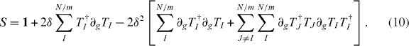
It is often the case that rather than the GSF, the GSF susceptibility, defined through Taylor expanding f up to O(δ2), f(x,δ;N) ≈ 1 − (δ2/2)χ(x;N), suffices to capture quantum criticality [6, 18]. Of course, this fidelity and susceptibility both depend on our choice of the embedding operator (or, in general, our QRG recipe). Expanding the embedding operator and using the identity T†(x)T(x) = 1 yields

Thus the above RG procedure for f applies to χ as well provided that we can treat S appropriately.
3. The Ising model in the transverse field
This model of a periodic chain of N sites is defined with the Hamiltonian

where J defines an energy scale, g is the parameter that controls QPT and σαi is the Pauli matrix for site i. To apply QRG, the chain is divided into blocks of m = 2 sites described by  , where hBI = −J(σz1,Iσz2,I + gσx1,I) [10]. The block–block interaction Hamiltonian is also represented by
  . hBI can be diagonalized exactly, whence TI is constructed from the two lowest eigenstates as
  , in which |ϕ1〉I = A(g)|↑↑〉 + B(g)|↓↓〉,|ϕ2〉I = A(g)|↑↓〉 + B(g)|↓↑〉 are the two degenerate ground states of hBI. Here {|↑〉,|↓〉} are the eigenvectors of σx,
  represent the states of block I, and
  ,
,  , with
  . The global embedding operator T = ⊗N/2I=1TI leads to
  , which is akin to the original one (equation (5)) modulo replacing the coupling constants with the renormalized couplings

The renormalized couplings after ℓ RG iterations are obtained simply from equation (6) upon substituting (J,g,J(1),g(1)) → (J(ℓ−1),g(ℓ−1),J(ℓ),g(ℓ)). We note that for this model the RG fixed points are ∈{0,1,∞}, from which gc = 1 is unstable whereas 0 and ∞ are stable under the RG flow (see figure 1).
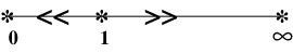
Figure 1. The RG flow diagram of the ITF model.
Download figure:
Standard imageA direct calculation of T†(g−)T(g+) shows that it satisfies the form of equation (2), whereby straightforward algebra shows that here

and

Thus through equation (3) one can find an analytical expression for fITF(g,δ;N). Figure 2 shows fITF(g,δ;N) for various values of (δ,N). A drop is seen at g = 1, which verifies it as a quantum critical point. In agreement with [19], two regimes  and Nδ⪆1, corresponding respectively to the 'small-size limit' and the 'large-size limit', can be discerned. In the small-size limit, the GSF drops at/around gc = 1, whereas in the large-size limit, the GSF drops to zero for a domain of gs around gc = 1 whose size is ≈O(δ) (figure 2 (right panel)).
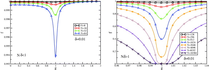
Figure 2. GSF of the ITF model versus the field strength g. Left: Small-size limit Nδ < 1. Right: large-size limit Nδ > 1.
Download figure:
Standard imageIn the thermodynamic limit, an interesting limit of the GSF can also be obtained. Note that the RG flow diagram (after equation (6)) indicates that there are three distinct regions to look at in the calculation of the GSF, because due to the RG flow g− and g+ may be carried away differently depending on the location of g and the value of δ (before applying the δ → 0 limit). Explicitly, these regions are: (i) g− < 1 and g+ < 1, (ii)  and g+ = 1, or g− = 1 and g+⪆1, (iii) g− > 1 and g+ > 1. One is usually interested in seeing how for a small (but nonvanishing) difference in the values of the parameters the associated ground states compare in the thermodynamic limit. This implies taking first the limit N → ∞ and next δ → 0. Thus, considering the RG flow diagram of the ITF model leads to

(where δg1 is the Kronecker delta function), which seems to be consistent with the small-size limit (figure 2 (left panel)). This sharp drop of the GSF is a signature that gc = 1 is a quantum critical point, consistent with what QRG suggests.
Note that the drop in the GSF accordingly signals a nonanalyticity in χITF, implying that here the GSF susceptibility is also reliable to identify the criticality of the model. In fact, expanding f(g,δ;N) up to O(δ2)—as explained in the formalism, equation (4)—yields the GSF susceptibility. Now, the S operator is given in the following form in terms of the block embedding operators:
For the ITF model, we obtain T†I∂gTI = 0 and ∂gT†I(g)∂gTI(g) = D(g)1, where D(g) = s2/[(1 + g2)(1 + s2)2]. Iterating the RG procedure leads to the following expression:

with ∂ℓ ≡ ∂g(ℓ), thence  . Note that g(ℓ) = g(ℓ−1) = gc = 1,
χ(ℓ)(1) = N2/32, hence χITF(gc) ∼ N2 [6]. For second-order QPTs, by using alternative methods such as quantum scaling analysis and the adiabatic theorem [8, 20, 21], it has been known that χ(gc) ∼ N2/dν, where d is the dimensionality and ν > 0 is the critical exponent capturing the divergence of the correlation length ξ ∼ |g − gc|−ν. Thus we obtain νITF = 1.
. Note that g(ℓ) = g(ℓ−1) = gc = 1,
χ(ℓ)(1) = N2/32, hence χITF(gc) ∼ N2 [6]. For second-order QPTs, by using alternative methods such as quantum scaling analysis and the adiabatic theorem [8, 20, 21], it has been known that χ(gc) ∼ N2/dν, where d is the dimensionality and ν > 0 is the critical exponent capturing the divergence of the correlation length ξ ∼ |g − gc|−ν. Thus we obtain νITF = 1.
Further scaling analysis can be done for fITF(g,δ;N) with fixed N or δ. Figures 3 and 4 show ln(−lnf) close to gc = 1 versus, respectively, ln δ for a fixed N = 32 768 and ln N for a fixed δ = 0.001, comparing the two ground states with g1 = 1 − kδ and g2 = 1 − (k + 1)δ, where k∈{0,1,2,3,4}. In figure 3, the k = 0 case, labeled by (1,1 − δ), comparing the ground state at the quantum critical point and a state very close to it in the ferromagnetic phase, shows behavior akin to the k ≠ 0 cases for small δs in the Nδ < 1 regime; however, it shows distinct behavior for Nδ > 1, signaling that one of the states is exactly at the quantum critical point. The k ≠ 0 cases, comparing in fact two states in the ferromagnetic phase close to the quantum critical point, exhibit lnf ∼ − δ2 scaling for Nδ < 1, connected with a crossover domain of Nδ ≈ O(1) to lnf ∼ − δ scaling for Nδ > 1, in agreement with [19]. In contrast, figure 4 exhibits lnf ∼ − N2.05 scaling for Nδ < 1, connected with a crossover domain of Nδ ≈ O(1) to the different lnf ∼ − N scaling for Nδ > 1, also in agreement with [19]. The distinct behavior of the (1,1 − δ) case suggests that one of the states is at the quantum critical point. The scaling behavior of the GSF around gc = 1 in the paramagnetic phase (g > 1) gives results similar to figures 3 and 4, which we have not presented here.

Figure 3. Scaling behavior of the GSF for the ITF chain with a fixed size N = 32 768: ln(−lnf) versus ln δ close to gc = 1.
Download figure:
Standard image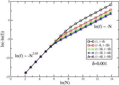
Figure 4. Scaling of the GSF for the ITF chain with a fixed δ = 0.001: ln(−lnf) versus lnN close to gc = 1.
Download figure:
Standard image4. The XXZ model
The anisotropic spin-1/2 Heisenberg (XXZ) model on an open chain is defined by [22]

where J > 0 is the exchange-energy coupling, Δ = (q + q−1)/2 is the axial anisotropy given in terms of a pure phase q, and

with a±(q) = (q ± q−1)/2. Equation (12) is different from the ordinary XXZ Hamiltonian in the boundary term ∝σz1 − σzN, which is unimportant in the thermodynamic limit. It is known that this model is critical (gapless) for |Δ| ⩽ 1 (critical line), exhibiting no long-range order [1].
The RG procedure here is implemented based on the quantum group property of the Pauli matrices [22]. The Hamiltonian (12) is decomposed to three-site blocks (m = 3), where the block I is composed of sites interacting as hBI = hiI,iI + 1 + hiI + 1,iI + 2, and the rest of the Hamiltonian constitutes the block–block interaction. The ground state of the block Hamiltonian is doubly degenerate, represented in the σz-basis as


where  . The embedding operator for block I is then given by
  , thereby T = ⊗ITI, where
  denote states of block I. Therefore, the renormalized Hamiltonian is obtained similarly to equation (12) with the following renormalized coupling constants:

By calculating T†(Δ−)T(Δ+)—after replacing equations (14) and (15)—we obtain that it satisfies the form of equation (2), where

where

Now through the RG formalism (especially noting that Δ(ℓ) = Δ), the following analytical expression is obtained for the GSF given any (Δ,δ;N):

Figure 5 represents this scaling for some values of Δ and δ.
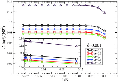
Figure 5. Average GSF susceptibility versus 1/N for the XXZ chain. In the inset the horizontal axis is a normal scale (unlike the log scale of the main plot). The behavior in the inset is reminiscent of figure 1 of [20] obtained through an exact diagonalization.
Download figure:
Standard imageInterestingly, this simple and elegant relation also enables detection of the associated criticality in the XXZ model (seen in [20, 23]), excluding conclusively doubts that the GSF might be insufficient [24]. Evidently, we have ω(ℓ) = ω(0) and |ω(ℓ)| < 1 for all δ ≠ 0 and |Δ| ⩽ 1; hence

That is, the entire |Δ| ⩽ 1 line is critical [1]. This is a remarkable result in that to characterize the criticality of the XXZ model we did not need to know the ground state or an approximation of that [20, 23]. We remark that the GSF susceptibility χXXZ = 6(N − 1)/[(1 − Δ2)(2Δ + 4)2], obtained through our RG approach, in contrast to the GSF, only captures the criticality at the symmetric point |Δ| = 1 (including the Kosterlitz–Thouless point Δ = 1 and the ferromagnetic critical point Δ = −1).
5. Summary
We have developed a viable, general QRG formalism to calculate GSF in quantum critical systems. Our formalism combines two powerful methods in a unified framework, enhancing the characterization of criticality in quantum many-body systems. Specifically, our formalism is structured on coarse-graining a quantum system (e.g. by partitioning it into blocks) and then rescaling the system length in order to eliminate short-scale or irrelevant interactions from the Hamiltonian. In various cases this enables a renormalization-based recurrence relation for the fidelity, without the need to know the system's ground state, an approximation thereof or an order parameter. With this advantage, one can utilize the QRG toolkit to boost or even simplify the calculation of critical properties in systems where renormalization works sufficiently well.
We have illustrated our formalism with two examples, the ITF and the anisotropic Heisenberg chain. In both models, our approach produced analytical expressions for the GSF, resulting in the expected criticality (especially in a simpler and more conclusive way than has already been suggested for the second model).
Applying our formalism to more sophisticated QPTs, such as nonintegrable two-dimensional models (although we did not use integrability throughout our formalism) or those featuring topological order, can be an interesting next direction to go. These seem viable in particular in light of results indicating that GSF is able to signal topological phase transitions, and that our formalism (at least explicitly) does not require exact solvability.
Acknowledgments
This work was partially supported by the Center of Excellence in Complex Systems and Condensed Matter at Sharif University of Technology. N Amiri, L Campos Venuti, H Johannesson and H-Q Zhou are acknowledged for comments on this work. AL acknowledges partial support from the Alexander von Humboldt Foundation.
Footnotes
- 4
Note that the QRG we work with is based on dynamics and not states; thus, in this respect, it differs from the formalism developed in [12].
- 5
A sufficient condition for this relation is that 〈ϕi(x−)|ϕi(x+)〉 = ω(x,δ), with some i-independent ω. This might be a manifestation of a selection rule associated with some symmetry.