


Abstract
We present a data analysis procedure that provides the solution to a long-standing issue in microrheology studies, i.e. the evaluation of the fluids' linear viscoelastic properties from the analysis of a finite set of experimental data, describing (for instance) the time-dependent mean-square displacement of suspended probe particles experiencing Brownian fluctuations. We report, for the first time in the literature, the linear viscoelastic response of an optically trapped bead suspended in a Newtonian fluid, over the entire range of experimentally accessible frequencies. The general validity of the proposed method makes it transferable to the majority of microrheology and rheology techniques.
Export citation and abstract BibTeX RIS

Content from this work may be used under the terms of the Creative Commons Attribution-NonCommercial-ShareAlike 3.0 licence. Any further distribution of this work must maintain attribution to the author(s) and the title of the work, journal citation and DOI.
1. Introduction
Since their first appearance in the 1970s [1], optical tweezers (OT) have been extensively developed and have proved to be an invaluable tool for a variety of applications throughout the biophysical sciences: e.g. they have been successfully employed for measuring the microrheology of a colloidal suspension [2], the compliance of bacterial tails [3], the forces exerted by a single motor protein [4], the mechanical properties of human red blood cells [5] and those of individual biological molecules [6–8].
From a mechanical point of view, OT can be considered as exceptionally sensitive transducers able to resolve pN forces and nm displacements, with high temporal resolution (down to μs). The physics underpinning the working principles of the OT relies on the ability of a focused laser beam to trap, in three dimensions, micron-sized dielectric particles suspended in a fluid [1, 9, 10]. The trapping process is achieved by optically guiding a (monochromatic) laser beam through a high magnification objective, with high numerical aperture, which also allows visualization of the micro-environment surrounding the trapped probe. The trapping force is generated by the combined action of both the gradient of the laser intensity profile and the difference between the refractive indexes of the materials constituting the fluid and the probe. OT are very often built around optical microscopes, like those commonly used for biological studies, and are equipped with a fast probe-position detector. The latter is usually chosen to be either a charge-coupled device camera [11] or a quadrant photodiode [12]; both of which provide the tracer trajectory with a spatial resolution of the order of nm [13], but the first has a detection rate upper limit of the order of kHz, while the second can reach rates of the order of MHz. Accessing the time-dependent trajectory of a micron sphere, to high spatial and temporal resolution, is one of the basic principles behind microrheology techniques [14, 15], as introduced hereafter. For a fairly comprehensive review on the state of art of OT setups and their applications, we refer the reader to [16–22] and those therein.
Microrheology is a branch of rheology, but it works at micron length scales and with micro-litre sample volumes. Therefore, microrheology techniques are revealed to be very useful tools for all those rheological studies where rare or precious materials are employed (e.g. in biomedical studies [23–25]). In addition, microrheology measurements can be performed in situ in an environment that cannot be reached by a bulk rheology experiment, for instance inside a living cell [26]. Microrheology techniques can be classified as either passive or active, depending on whether they monitor respectively the free or the driven motion of tracer particles introduced in the fluid under investigation. In the first case, the tracers' motion is governed by the thermal fluctuations of the surrounding fluid's molecules; whereas in the second case, an external force field is applied to the tracers. In the past decades, many microrheology techniques have been developed, including video particle tracking microrheology [27], diffusing wave spectroscopy [28, 29], atomic force microscopy [30], magnetic tweezers [31, 32] and OT [33–39]. For a good overview and understanding of the historical roots of the most common microrheology techniques, the reader is referred to [15, 40–42]. In general, microrheology techniques are aimed at relating the time-dependent tracers' trajectories to the linear viscoelastic (LVE) properties of the fluid in which they are dispersed.
The LVE properties of a material can be represented by the frequency-dependent complex shear modulus G*(ω), which provides information on both the viscous and the elastic nature of the material. This is defined as the ratio between the Fourier transforms (denoted by the symbol '  ') of the stress σ(t) and the strain γ(t) [43], regardless of which has been imposed and which has been measured:

where ω is the angular frequency and i is the imaginary unit (i.e. i2 = −1). The conventional method of measuring G*(ω) is based on the imposition of an oscillatory stress σ(ω,t) = σ0 sin(ωt) (where σ0 is the amplitude of the stress function) and the measurement of the resulting oscillatory strain, which would have a form like γ(ω,t) = γ0 sin(ωt + δ(ω)), where γ0 is the strain amplitude and δ(ω) is the frequency-dependent phase shift between the stress and the strain; from equation (1) it follows that

where G'(ω) and G''(ω) represent the material storage (elastic) and loss (viscous) moduli, respectively. For example, in the case of a purely elastic solid, the stress and the strain are in phase and δ(ω) = 0 → G*(ω) ≡ G'(ω); whereas, for a purely viscous fluid, such as water or glycerol, δ(ω) = π/2 → G*(ω) ≡ iG''(ω). For complex solids (e.g. gels, rubbers) or viscoelastic fluids (e.g. oil [44], saliva [45]) δ(ω) would take any value between the above limits (i.e. 0 ⩽ δ(ω) ⩽ π/2) depending on the frequency at which the stress or the strain is applied. Note that G*(ω) is time invariant.
In this paper we provide the solution to a long-standing issue in microrheology studies, i.e. the evaluation of the fluids' LVE properties from the analysis of a finite set of experimental data, describing (for instance) the time-dependent mean-square displacement (MSD) of suspended probe particles experiencing Brownian fluctuations [14, 46–53]. In particular, we tune the analytical method introduced by Evans et al [54], for converting creep compliance J(t) (a function simply proportional to the MSD) into G'(ω) and G''(ω), to microrheology measurements performed with OT. We report, for the first time in the literature, the LVE response of an optically trapped bead suspended in a Newtonian fluid, over the entire range of experimentally accessible frequencies; both for synthetic and real experimental data. In addition, we present an improved method to evaluate the frequency-dependent complex shear modulus G*(ω) of generic fluids including water-based solutions of F-actin protein. The general validity of the proposed method makes it transferable to the majority of microrheology techniques.
The paper is organized as follows. In section 2 we describe the apparatus used. In section 3, we discuss the theoretical background required to obtain rheological data from OT. In section 4, we discuss novel methods of data analysis that avoid the introduction of artefacts. We anticipate some results for a relevant biological fluid (i.e. solutions of actin filaments) in section 5, and draw conclusions in section 6.
2. Apparatus
Optical trapping is achieved by means of a titanium-sapphire laser with a 5 W pump (Verdi V5 laser; Coherent Inc.), which provides up to 1 W at 830 nm. The tweezers are based around an inverted microscope, where the same objective lens (100 × , 1.3 numerical aperture, Zeiss, Plan-Neofluor) is used both to focus the trapping beam and to image the thermal fluctuations of either a 2 or 5 μm diameter silica bead. Samples are mounted on a motorized microscope stage (Prior Pro-Scan II). A complementary metal-oxide semiconductor camera (Dalsa Genie HM640 GigE) takes high-speed images of a reduced field of view. These images are processed in real-time at ≈1 kHz using our own LabVIEW (National Instruments) particle tracking software [55] running on a standard personal computer.
3. Theoretical background
When a micron-sized spherical particle is suspended in a fluid at thermal equilibrium, it experiences random forces leading to Brownian motion, driven by the thermal fluctuations of the fluid's molecules. Analysis of the particle's trajectory reveals information on the viscoelastic properties of the suspending fluid, as demonstrated in the pioneering work of Mason and Weitz [14] that established the field of microrheology. In particular, they showed that, at thermal equilibrium, the trajectory  of a naturally buoyant bead is directly related to the LVE properties of the surrounding complex fluid by means of a generalized Langevin equation

where m is the mass of the particle,  is its acceleration,
  its velocity and
  is the usual Gaussian white noise term, modelling stochastic thermal forces acting on the particle. The integral term, which incorporates a generalized time-dependent memory function ζ(t), represents viscous damping by the fluid. Using the assumption that the Laplace-transformed bulk viscosity of the fluid
  is proportional to the microscopic memory function
  , where a is the bead radius, they provided the solution to equation (3) in terms of the MSD:

where kB is Boltzmann's constant, T is absolute temperature and  is the Fourier transform of the MSD
 ![$\langle \Delta r^2(\tau )\rangle \equiv \langle [\vec {r}(t+\tau )-\vec {r}(t) ]^{2} \rangle $](https://content.cld.iop.org/journals/1367-2630/14/11/115032/revision1/nj433868ieqn9.gif) . The average
. The average  is taken over all initial times t and all particles, if more than one is observed.
In the case when the probe's fluctuations are constrained by a stationary harmonic potential generated by OT, one could write a generalized Langevin equation similar to equation (3), but with an additional term accounting for the trapping force:

Here, κ is the OT trap stiffness, which can be easily determined by appealing to the principle of equipartition of energy:

where 〈r2j〉 is the time-independent variance of the Cartesian component (j = x,y,z) of the d-dimensional vector describing the particle's displacement from the trap centre, the origin of  . Note that, for non-symmetric traps (i.e. κ ≠ κj,∀j) equation (5) is still valid but in one dimension, with κ replaced by κj evaluated for each component. Despite the great variety of methods for determining the trap stiffness (e.g. using the power spectrum or the drag force [18, 56, 57]), equation (6) provides the only such measurement that is independent of the viscoelastic properties of the fluid under investigation and is thus essential for proper calibration. This is because, whatever the elasticity of the unknown fluid, its contribution to the time-independent constraining force must vanish at long lag-times (because at rest the fluid's elastic shear modulus goes to zero as the time goes to infinity). Thus the trap stiffness is easily determined by means of equation (6) applied to a sufficiently long measurement (i.e. longer than the fluid's longest relaxation time) via the evaluation of the time-independent variance of the confined particle position.
Following the same assumptions made by Mason and Weitz for the case of freely diffusing particles, equation (5) can be solved in terms of either the normalized mean-square displacement (NMSD)  [36] or the normalized position autocorrelation function (NPAF)
  [37]:
[37]:

where  and
and  are the Fourier transforms of Π(τ) and A(τ), respectively. The inertial term (mω2), present in the original publications [36, 37], has been neglected here because, for micron-sized particles, it only becomes significant above the MHz frequency range. The quantities A(τ) and Π(τ) are simply related to each other [37]:

In addition, by Fourier transforming equation (8) one obtains the relation:  , which will prove useful later in the manuscript. The relationships between measurements made in the presence or absence of an OT are further reviewed in the appendix.
In principle, equations (4) and (7) are simple expressions relating the material's complex shear modulus G*(ω) to the observed time-dependent bead trajectory  via the Fourier transform of one of the related time-averaged quantities. In practice, the evaluation of these Fourier transforms, given only a finite set of data points over a finite time domain, is non-trivial since interpolation and extrapolation from those data can yield artefacts that lie within the bandwidth of interest.
The first attempt to address this issue for microrheology [14] was to fit the measured  to a preconceived functional form, and then use analytic continuation (swapping Laplace for Fourier frequency, s → i ω) to recover G'(ω) and G''(ω). A later approximate method [51] recovered the moduli from the log slope of the MSD, without numerical inversions, and was subsequently improved upon [52] by accounting for curvature.
An alternative method has been proposed by Evans et al [54] to convert creep compliance J(t) (and therefore MSD) into G'(ω) and G''(ω) directly, without transforms or fitting functions. This method is based on the interpolation of the finite data set by means of a piecewise-linear function. The general validity of the proposed procedure makes it equally applicable to find the Fourier transform  of any time-dependent function g(t) that vanishes for negative t, sampled at a finite set of data points (tk,gk), where k = 1,...,N, which extend over a finite range, and need not be equally spaced [54]:
where  is the gradient of g(t) extrapolated to infinite time and g(0) is the value of g(t) extrapolated to t = 0 from above.
4. Data analysis
Although equation (9) has been successfully employed in both classical bulk rheology [58, 59] and microrheology studies [32, 36, 37, 53], when it is applied to microrheology measurements performed with OT, there remain two issues, common to all the other methods described above, that compromise the quality of the results. Nevertheless, we shall introduce a data analysis procedure that markedly reduces the undesired effects of these experimental issues, providing a useful tool for microrheology.
4.1. Interpolation artefacts
The first issue is related to the Nyquist–Shannon sampling theorem [60]: 'If a function contains no frequencies higher than W cps, it is completely determined by giving its ordinates at a series of points spaced 1/(2 W) seconds apart'. Conversely, we cannot expect to recover complete information about the fluid's LVE properties from the Fourier transform of a discrete data set (e.g. MSD, NMSD or NPAF) at frequencies higher than one half of the data acquisition rate (AR) if the rate is uniform. Above that frequency, the information in the Fourier transform is artificial, describing the details of the interpolation scheme between the data points. Unfortunately, those artefacts will almost certainly spread some way below the Nyquist limit, contaminating the experimental results. This occurs due to the broad spectrum of the sharp corners between straight-line segments in the interpolation scheme used to derive equation (9).
This first issue is simply resolved by virtually oversampling the time-averaged functions (e.g. Π(τ)) that contain the fluid's LVE properties. Oversampling is a very common procedure in signal processing and it consists of sampling a signal with a sampling frequency fs much higher than the Nyquist rate 2B, where B is the highest frequency contained in the original signal. A signal is said to be oversampled by a factor of β ≡ fs/(2B) [61]. Microrheological measurements performed with OT have a maximum value of B limited by the detector's AR. We choose to oversample by interpolating the measured time-averaged functions (e.g. A(τ)) with a natural cubic spline, which is piecewise cubic and twice continuously differentiable.
Having generated the larger over-sampled data set from the original data set, it remains important to use equation (9) to find its Fourier transform, since that equation correctly assumes causality (the function vanishes for negative time), extrapolates to infinite time (using the parameter  ) and guarantees that no other assumptions bias the data. In contrast to our cubic-spline interpolation, a fitting procedure based on preconceived models would doctor the experimental results; our interpolation procedure preserves the original data within the bandwidth limits imposed by the sample rate. Note that, following the oversampling and conversion, the resulting rheological data (the frequency-dependent viscoelastic moduli) should only be examined at frequencies within the experimentally valid frequency window, since no real information exists above the Nyquist frequency. We shall show that this data-analysis procedure yields artefact-free results right up to the Nyquist limit.
To validate the solution to this first issue, we initially apply it to a simple analytical example NPAF, in the form of a single exponential decay: A(τ) = e−λτ, where λ = κ/(6πaη), as if obtained from infinitely long measurements of the thermal fluctuations of a particle harmonically trapped in a Newtonian fluid. This is the dynamic response of an ideal Kelvin–Voigt material (see equation (A.6)), for which the frequency spectrum is known to have a simple analytical form (equation (A.7)). Defining the normalized complex modulus  and substituting the Kelvin–Voigt NPAF into equation (7) yields

where  .
.
In figure 1 (left) we report an example in which the idealized NPAF has been sampled at a frequency of fs = 1 kHz, as if it were obtained from thermal fluctuations of a 5 μm diameter sphere constrained by an OT with trap stiffness of κ = 1 μN m−1 and suspended in a Newtonian fluid of viscosity η = 0.896 mPa s, where the bead trajectory had been acquired at AR ≡ fs and for an infinite time, up to a lag-time of 1 s. We reconstruct the dynamic response of the system via equation (A.6), with the Fourier transform of A(τ) evaluated by means of equation (9); the results are shown in figure 1 (right). It is clear that artefacts in the frequency domain, where  starts to diverge from its expected value (due to the finite sampling rate and implicit piecewise-linear interpolation in the time domain), begin at ω ≃ λ (i.e.
  ), whereas,
  starts to deviate from its expected value (i.e.
  ) only at ω ≃ 20λ.

Figure 1. (Left) The NPAF  versus lag-time, where λ = κ/(6πaη) ≃ 24 s−1. The NPAF has been built using the following parameter values: fs = 1 kHz, κ = 1 μN m−1, a = 2.5 μm, η = 0.896 mPa s. The inset shows the same data as above, but with the semi-log representation of the axis inverted. (Right) The normalized complex modulus versus frequency evaluated via equation (7) and by means of equation (9) applied to the data shown on the left; both quantities are dimensionless.
Download figure:
Standard imageFigure 2 demonstrates that the correct values of the LVE moduli are recovered by oversampling the discrete data shown in figure 1 (left) to a sufficiently high value of β ≡ fs/(2AR) ≫ ω/AR, using a natural cubic spline interpolation. Here, we have taken fs≅8.2 MHz, implying β≅4100. Note that a detailed study of the errors in evaluating the moduli as a function of β is reported in the appendix. In figure 2, both the moduli now show the expected values (i.e. equation (10)) over the entire range of explored frequencies.
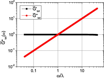
Figure 2. The normalized complex modulus versus frequency evaluated via equation (7) and by means of equation (9) applied to the data shown in figure 1 (left), but interpolated with a natural cubic spline function having fs≅8.2 MHz. This correct normalization confirms the validity of the data analysis method.
Download figure:
Standard image4.2. Noise
The second issue relates to the accuracy with which the data (i.e. 〈Δr2(τ)〉, Π(τ) or A(τ)) are evaluated, especially at long lag-times. Indeed, since all the functions of particle position in equations (4) and (7) are time-averaged quantities, they become exact only in the limit of infinite measuring time (or equivalently for N → ∞), which is unachievable in reality.
In order to quantify the uncertainty of a time-averaged function (measured over a finite set of data) with respect to its expected value, we have evaluated the MSD of 104 simulated trajectories of freely diffusing particles, with each trajectory comprising 106 random steps, drawn from a uniform distribution of unit width; so that, e.g. the MSD at lag-time τ = 1 has been evaluated over ∼1010 displacements. The resulting curve shown in figure 3 satisfies the expectation that MSD ∝τ. However, within a single trajectory of 106 steps the error in the measured MSD, for a lag-time of 104 time units is typically as large as 10%. As shown in figure 3, the percentage deviation of the MSD(τ) from its expected value for each trajectory grows with lag-time, as a power law close to τ1/2.

Figure 3. (Left axis) The MSD versus lag-time of 104 simulated trajectories of freely diffusing particles; each trajectory is made up by 106 data points (i.e. steps). (Right axis) The percentage deviation of the MSD from its expected value for each trajectory.
Download figure:
Standard imageIn real experiments this uncertainty affects the results in the following way. Since the Fourier transform is an integral operator, all the short time-scale deviations of the measured time-averaged function from its expected value will communally contribute noise to the results at high frequencies, especially those occurring at long lag-times where the averages are inexorably less accurate. This is clearly shown in figure 4 (left), where the agreement between the measured NMSD and its prediction, via equation (A.5), is very good at small lag-times; whereas it becomes worse at long lag-times (see the inset of figure 4 (left)). Although all of the data contribute to the high-frequency noise, the high-frequency signal derives predominantly from the measurements at short lag-times. In long-duration experiments, this signal can become swamped by noise from the large quantity of long lag-time data. A simple but crude solution to this problem, to improve the signal-to-noise ratio, is obtained by reducing the data density (i.e. the sampling rate) at long lag-times. This is achieved by evaluating the time-averaged functions (e.g. A(τ)) at values of τ that are logarithmically (or near-logarithmically) distributed on the time-scale, as shown in figure 4 (right). In this particular case, we have evaluated (or sampled) A(τ) at lag-times τn = ceil(1.45n), for non-negative integer n (where ceil(...) is the ceiling function, which rounds the input variable to the next highest integer); so that, the first five points are linearly spaced in time, whereas all the others are logarithmically distributed. In this way, we enhance the relative statistical weight of the reliable data at short lag-times and substantially reduce the number of disruptive short time-scale deviations of A(τ) from its expected value, occurring at long lag-times.

Figure 4. (Left) Comparison between the Π(τ) (circles) and its prediction (continuous line), via equation (A.5), for an optically trapped 4.74 μm diameter silica bead suspended in water, with κ = 0.93 μN m−1 and η = 0.896 mPa s. The NMSD has been obtained from the analysis of 106 data points representing the particle trajectory, acquired at AR ≃ 1 kHz. The inset highlights the behaviour of Π(τ) within a small time-window taken at long lag-times. (Right) The same data as shown on the left, but plotted in terms of the NPAF versus lag-time (circles); whereas the red square symbols represent the same data as before, but sampled at lag-times quasi-logarithmically distributed on the time-scale: τn = ceil(1.45n), for non-negative integer n.
Download figure:
Standard imageFinally, we apply both the above techniques to analyse real experimental data, to yield the full viscoelastic spectrum of optically trapped micro-spheres suspended in Newtonian fluids. In figure 5 (left) we report the NPAF of optically trapped spheres suspended in both water and 20% w/w glycerol/water mixture while, in figure 5 (right), we report the real and imaginary parts of the normalized complex modulus evaluated via equation (A.6) and by means of equation (9) applied to the sampled data shown in figure 5 (left) after interpolation with a natural cubic spline function having fs = 25 and ≃3.7 MHz, respectively. From figure 5 (right) it is clear that, although there remains some noise in the real component of the complex modulus at high frequencies, the agreement between the results and the expected values (i.e. equation (10)) is very good.
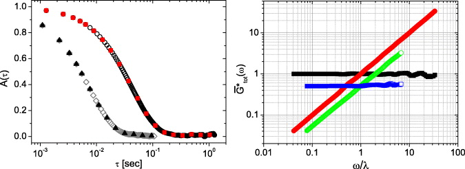
Figure 5. (Left) Comparison between the NPAF shown in figure 4 (circles) with that obtained from the analysis of an optically trapped 2 μm diameter silica bead suspended in 20% w/w glycerol/water mixture (diamonds), with κ = 4 μN m−1 and η = 1.6 mPa s. Both the NPAFs have been sampled at lag-times quasi-logarithmically distributed on the time-scale: τn = ceil(1.45n), for non-negative integer n (squares and triangles, respectively). (Right) The normalized complex modulus versus frequency (both dimensionless) evaluated via equation (7) and by means of equation (9) applied to the sampled NPAFs shown on the left, but interpolated with a natural cubic spline function having fs = 25 and ≃3.7 MHz, respectively. Note that, the normalized moduli obtained from the glycerol/water mixture (i.e.  , blue open square symbols, and
  , green open circle symbols) have been scaled by a factor of two for a clearer visualization. The black square and the red circle symbols represent the normalized moduli for the measurement performed with water.
Download figure:
Standard imageBased on these results, we can confirm that the OT acts as a linear force transducer when operating in the range of frequencies up to ∼kHz and on micron-sized particles (i.e. when the laser wavelength is smaller than the particle diameter). However, it is important to be aware that, under other operating conditions, the OT response may not remain linear [62–65].
5. Results for solutions of actin filaments
Having established the efficacy of the new method of data analysis, we use it to obtain clean, artefact-free viscoelastic moduli of an important biological fluid, for which conventional rheology is difficult due to the sample volumes available. In particular, we anticipate some results from an OT based microrheology study performed on solutions of actin filaments, reminding that more detailed bio-physical studies of these solutions will be presented elsewhere.
The cytoskeleton is a network of protein-fibres that runs throughout the matrix of living cells. It provides a framework for organelles, anchors the cell membrane, facilitates cellular movement and provides a suitable surface for chemical reactions to occur. The cytoskeleton is made up of three types of protein filaments: microfilaments (also called thin filaments), intermediate filaments and microtubules. The mechanical properties of thin filament networks control specific biological functions (e.g. regulation of muscle contraction), but these mechanical properties are difficult to measure in vivo. This problem has motivated an extensive research effort to investigate the mechanical properties and microstructure of reconstituted thin filament networks in vitro [66–69]. At low ionic strength in vitro, actin exists in the monomeric (globular) G-actin form. G-actin is roughly spherical with a diameter of about 5 nm. When the ionic strength of a G-actin solution is increased to a physiological value (0.1 M), G-actin self-associates to form the backbone of the thin filament—the actin filament (F-actin), which can be viewed as either a two-stranded long-pitch (≃37 nm) helical structure or a single short-pitch (≃5.9 nm) helical structure [70], which is related to the size of the monomeric G-actin.
F-actin is a biological example of a semi-flexible polymer that is characterized by a persistence length ranging from ∼2 to ∼30 μm [71–73] and a diameter of ≃8 nm [71, 74]. Despite their importance to biophysical studies, the viscoelastic properties of semi-flexible polymer solutions are still not well understood and a basic analytical model has not yet been agreed upon; thus the need of accurate experimental data describing the rheological properties of semi-flexible polymer solutions to inform the development of theoretical models.
In figure 6 (left) we report the NPAF of an optically trapped 5 μm diameter silica bead suspended in a solution of F-actin at concentration of 0.1 mg ml−1. The inset shows the short time-scale deviations occurring at long lag-times because of the poor accuracy to which A(τ) can be evaluated from a finite-size data set representing the particle trajectory  (here 106 data points). Figure 6 (right) shows the LVE properties of the F-actin solution evaluated via equation (7) and by means of equation (9) applied to the sampled A(τ) after interpolation with a natural cubic spline function with fs = 12 MHz. At high frequencies, both moduli are in good agreement with the theoretical predictions: G'(ω)∝ω3/4 and G''(ω)∝ω7/8. Indeed, while the former power-law is an archetype for the dynamics of semi-flexible polymer solutions [75, 76], the latter is not so commonly observed, although predicted by Everaers et al [77], Liverpool [78] and, more recently [79, 80], in models that combine the effects of both longitudinal and transverse fluctuations on the dynamics of a semi-flexible filament. They found that, at short times, the fluctuations perpendicular to the local axis of the polymer scale as
  (similarly found by Morse [76]), while fluctuations parallel to the local axis follow a different law
  and are correlated over a length l∥∝t1/8.
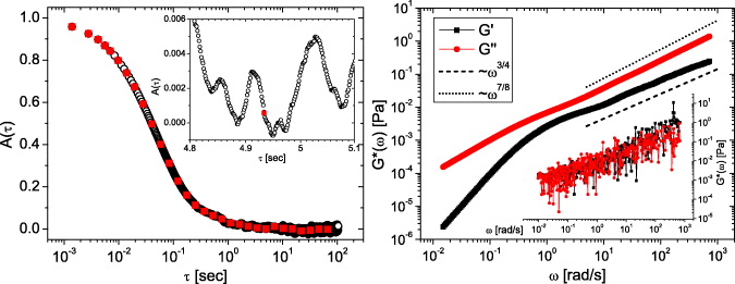
Figure 6. (Left) (Circles) The NPAF versus lag-time of an optically trapped 5 μm diameter silica bead suspended in a solution of F-actin at concentration of 0.1 mg ml−1 and κ = 2.8 μN m−1. The NPAF has been evaluated from a trajectory made up by 106 data points. (Squares) Same data as before, but sampled at lag-times quasi-logarithmically distributed on the time-scale: τn = ceil(1.45n), for non-negative integer n. The inset shows the disruptive short time-scale deviations occurring at long lag-times. (Right) The complex modulus versus frequency evaluated via equation (7) and by means of equation (9) applied to the sampled NPAF shown on the left, but interpolated with a natural cubic spline function having fs = 12 MHz. The lines are guides for the gradients. The inset shows the disruptive effects of the short time-scale deviations occurring at long lag-times when the G*(ω) is evaluated via equation (7) and by means of equation (9) directly applied to the original NPAF shown on the left.
Download figure:
Standard image
Figure 7. Schematic representations of Jtot(t) (∝Π(τ), see equation (A.4)) for the cases of a trapped spherical particle suspended in both a Newtonian fluid and a generic viscoelastic fluid.
Download figure:
Standard image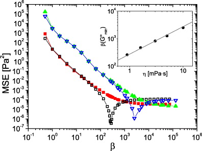
Figure 8. The mean-square error (MSE) of the viscoelastic moduli (from their expected values) versus the oversampling ratio β derived from the analysis of two NPAF having the form of a single exponential decay: A(τ) = e−λτ, where λ = κ/(6πaη), κ = 1 μN m−1, a = 2.5 μm, η = 0.896 mPa s (squares) and η = 10 mPa s (triangles), respectively. The filled and the open symbols refer to the MSE for G' and G'', respectively. The inset shows the relationship between β, taken where the MSE for G'' is minimum, and the viscosity of the Newtonian fluid (i.e. η = 0.896,1.6,3,5 and 10 mPa s). The line is a guide for the gradient (i.e. β(G''min)∝η).
Download figure:
Standard image6. Conclusions
An improved data analysis procedure for determining the LVE properties of complex fluids has been successfully applied to microrheology measurements with OT. The reliability of the novel data analysis procedure has been tested by evaluating the LVE response of optically trapped beads suspended in Newtonian fluids. For the first time in the literature, the frequency-independent elastic component of an optical trap has been measured over the entire range of experimentally accessible frequencies. The general validity of the proposed method makes it transferable to the majority of microrheology and rheology techniques.
Acknowledgments
We thank Francesco Greco and Miles Padgett for helpful conversations. MT acknowledges support via personal research fellowship from the Royal Academy of Engineering/EPSRC. We are grateful to EPSRC and BBSRC for supporting this work through grants EP/F040857/1 and BB/C511572/1, respectively, and to the DTC in Proteomic and Cell Technologies (EPSRC) for funding RLW.
Appendix A.: Rheological characterization of optical tweezers
It is worthwhile reviewing some fundamental relationships between the most common parameters describing the materials' LVE properties and the time-averaged functions (e.g. MSD) derived by analysis of the particle's thermal fluctuations. Let us begin by describing a simple relationship between the MSD of a freely diffusing particle and the time-dependent compliance J(t) of the suspending fluid. In classical rheology (i.e. in shear flow), the creep compliance is defined as the ratio of the time-dependent shear strain γ(t) to the magnitude σ0 of the constant shear stress that is switched on at time t = 0: J(t) = γ(t)/σ0. The latter is related to the shear relaxation modulus G(t) by a convolution [43]

Since the complex shear modulus G*(ω) (i.e. equation (1)) is the Fourier transform of the time derivative of G(t), by taking the Fourier transform of equation (A.1) it follows that

where  and
and  are the Fourier transforms of G(t) and J(t), respectively. By equating equations (A.2) and (4) one obtains

where it has been assumed that the inertial term (mω2) in equation (4) is negligible for frequencies ≪MHz and that J(0) = 0 for viscoelastic fluids. Equation (A.3) expresses the linear relationship between the MSD of suspended spherical particles and the macroscopic creep compliance of the suspending fluid [81].
Let us now consider an optically trapped spherical particle suspended in a viscoelastic fluid. For such a system, equation (A.3) would still hold, but it would describe the relationship between the measured MSD of a constrained particle and the compliance (Jtot) of the compound system made up of the optical trap and the viscoelastic fluid:

where the second expression follows from equations (6) and (8). In the simplest case where κ ≡ κj∀j (j = x,y,z), d = 3 and the suspending fluid is Newtonian, with a time-independent viscosity η, the compound system (OT plus fluid) can be modelled as an ideal Kelvin–Voigt material, with elastic constant proportional to the trap stiffness, κ/(6πa), and viscosity equal to η. In this case, Jtot assumes a simple analytical form

where λ = κ/(6πaη) is the relaxation rate of the compound system, known as the corner frequency when the thermal fluctuations of an optically trapped bead are analysed in terms of the power spectral density [56]. In practice, λ defines a characteristic time (t* = λ−1) at which the fluid compliance (J(t) = t/η(t)) equals the compliance of the optical trap (JOT = 6πa/κ): J(t*) = JOT; as schematically shown in figure 7, where the intersection of J(t) and JOT identifies t*.
Finally, from equations (A.2) and (A.4), one can also express the viscoelastic properties of the compound system in the frequency domain:

which, for a system modelled as an ideal Kelvin–Voigt material, becomes

In summary, the LVE properties of a generic viscoelastic fluid can be obtained by subtracting the frequency-independent elastic contribution of the optical trap from equation (A.6): G*(ω) = G*tot(ω) − κ/(6πa); notably, this is the same expression as the one reported in equation (7), but the latter has been derived from a more rigorous analytical procedure [36, 37]. Moreover, it is important to highlight that in [36, 37], Tassieri et al introduced two simple experimental procedures, coupled with data analysis methods, for determining the wideband viscoelastic properties of complex fluids in measurements involving OT. Those experimental procedures are still valid as they overcame the intrinsic issue of microrheology measurements performed with static OT, i.e. the loss of information on low-frequency viscoelastic properties of fluids with relaxation times longer than t*. In such cases, the OT compliance overshadows the fluid compliance (see figure 7) at long times (i.e. low frequencies); hence the need for either of the methods introduced in [36, 37].
Appendix B.: β-parameterization of the errors
In order to better understand the implications related to the choice of the oversampling ratio β on the Fourier transform of a generic function (e.g. A(τ)) via equation (9), we evaluate the MSE of the viscoelastic moduli (from their expected values) derived from the analysis of a NPAF having the form of a single exponential decay: A(τ) = e−λτ, where λ = κ/(6πaη), as already described in the main body of the paper (e.g. see figure 1 (left)) and for which the frequency spectrum is known to have a simple analytical form (i.e. equation (A.7)).
In figure 8 we report the results obtained from the analysis of the MSE of both the moduli as a function of β for five systems differing from each other only for the viscosity values of the fluids (i.e. κ and a are kept constant, whereas η = 0.896, 1.6, 3, 5 and 10 mPa s). All five systems give similar behaviour as for the two cases shown in figure 8 (note that, not all of the curves have been shown for clarity of the graph), i.e. the MSE decreases substantially as β increases up to a value of the order of β ≈ 103, after which it tends to stabilize around values of the order of ≈1E−5 and ≈1E−4 for G' and G'', respectively. Therefore, within a single measurement, a further increase of β above the value of ≈103 would not induce substantial improvement of the results. Moreover, it is interesting to highlight the feature shown by the MSE curves of G'' for all five systems, i.e. they clearly exhibit a minimum before reaching the plateau at higher values of β. The inset of figure 8 shows the quasi-linear relationship between β, taken where the MSE for G'' is minimum, and the viscosity of the Newtonian fluid. The non-trivial behaviour of this error is worthy of further study.